Introduction

About the Project

This repository contains some of the most intriguing and awesome algorithms of daily life implemented in languages primarily in C/C++/Java/Python.

Project Details

The entire project is divided into 4 parts

Competitive Coding Algorithms and Data Structures
Security Algorithms
Machine Learning Algorithms
Statistical / Mathematical Algorithms

Algebra

Sieve of Eratosthenes

Sieve of Eratosthenes is an algorithm that helps us find all the prime numbers in a range $[1, n]$. Initially, we take a boolean array of size $n+1$ where the $i$'th index will be true if $i$ is prime, and false otherwise. All the numbers except 0 and 1 are marked as prime at the beginning of the process.

Then we loop through the numbers from 2 till $n$ and if the number is currently marked as prime, then we add that number to our list of primes and mark all it's multiples as non-prime. At the end of the process, we will have all the prime numbers in the range in our list.

Let us try to simulate the process for $n=16$. The numbers will be placed between brackets in the diagrams if they are marked as non-prime. Initially, all numbers are marked prime except 1.

(1) 2 3 4 5 6 7 8 9 10 11 12 13 14 15 16

Now, the loop variable, say $i$, is at 2, which is a prime, so we mark all it's multiples as non-prime.

(1) 2 3 (4) 5 (6) 7 (8) 9 (10) 11 (12) 13 (14) 15 (16)

We do the same for i=3.

(1) 2 3 (4) 5 (6) 7 (8) (9) (10) 11 (12) 13 (14) (15) (16)

One important observation here is that all non-prime numbers are marked within $\sqrt{n}$ iterations. So, we can go through the remaining numbers and add them if they are prime. So the primes in the range would be: [2, 3, 5, 7, 11, 13].

Implementation

C++

vector<int> get_primes(int n)
{

    vector<int> primes;
    vector<bool> is_prime(n+1, true);
    is_prime[0] = is_prime[1] = false;

    for(int i=2; i<=n; i++)
    {
        if (!is_prime[i])
            continue;
        primes.push_back(i);
        for(int j=i*i; j<=n; j+=i)
            is_prime[j] = false;
    }
    return primes;
}

Python

def SieveOfEratosthenes(n):
    isPrime = [True]*(n+1)
    isPrime[0] = isPrime[1] = False
    primes = []
    for i in range(2, n+1):
        if not isPrime[i]:continue
        primes += [i]
        for j in range(i*i, n+1, i):
            isPrime[j] = False
    return primes

Other than finding primes, the algorithm can also be used to factorise any number less than or equal to $n$ in O(divisors) time if we simply store the smallest prime factor of each number in the array.

Practice Problems

Fibonacci Sequence

Introduction

The Fibonacci sequence is defined using the following recurrence relation:

$F_n = F_{n-1} + F_{n-2}$

where, $F_0 = 0, F_1 = 1$. This simple recurrence can be used to calculate $n$'th fibonacci number in $O(n)$ time.

Binet's Formula

Binet's formula is an explicit formula used to find the nth term of the Fibonacci sequence.

$F_n = \frac{\left(\frac{1 + \sqrt{5}}{2}\right)^n - \left(\frac{1 - \sqrt{5}}{2}\right)^n}{\sqrt{5}}$

Note that the absolute value of the second term is less than 1, so as $n$ increases, it's value tends to 0. Thus, we can say that the value of the first term alone is nearly equal to F_n. The formula also requires very high accuracy and is therefore not practical for larger values of $n$.

Matrix Form

Consider the following relation:
$\begin{pmatrix}F_{n-1} & F_{n} \cr\end{pmatrix} = \begin{pmatrix}F_{n-2} & F_{n-1} \cr\end{pmatrix} \cdot \begin{pmatrix}0 & 1 \cr 1 & 1 \cr\end{pmatrix}$

Then,

$\begin{pmatrix}F_n & F_{n+1} \cr\end{pmatrix} = \begin{pmatrix}F_0 & F_1 \cr\end{pmatrix} \cdot P^n$

where, $P \equiv \begin{pmatrix}0 & 1 \cr 1 & 1 \cr\end{pmatrix}$

$P^{n}$ can be calculated in $O(\log{n})$ time using matrix exponentiation. This particular method of calculating $n$'th Fibonacci term is useful when $n$ is very large, and the result is needed modulo some integer $m$.

Python

multiply = lambda A, B, mod: [[sum(i * j for i, j in zip(row, col)) % mod for col in zip(*B)] for row in A]

def f(n, m):
    p = [[0, 1], [1, 1]]
    result = [[1, 0], [0, 1]]
    cur = 1
    i = 0
    while cur <= n:
        if n & (1<<i):
            result = multiply(result, p, m)
        i += 1
        cur *= 2
        p = multiply(p, p, m)
    return multiply([[0,1]], result, m)[0][0]

Practice Problems

References

CP-Algorithms

Linear Diophantine Equations

Introduction

A linear diophantine equation is one of the form $ax + by = c$, where $a$, $b$ and $c$ are integers known to us. A solution to the equation will exist only when $\gcd(a,b)$ divides $c$, where gcd denotes the greatest common divisor.

To find one of the solutions, we can apply the extended Euclidean algorithm to find the gcd of $a$ and $b$, and two numbers $x_{g}$ and $y_{g}$ such that $ax_{g} + by_{g} = g$.

The implementation is as follows:

C++

pair<int, int> solve(int a, int b, int c)
{
    int m1=1, m2=0, n1=0, n2=1;
    while (a % b)
    {
        int quotient = a / b;
        int remainder = a % b;
        int aux1 = m1-(m2*quotient);
        int aux2 = n1-(n2*quotient);
        a = b;
        b = remainder;
        m1 = m2;
        n1 = n2;
        m2 = aux1;
        n2 = aux2;
    }
    return make_pair(m2*c,n2*c);
}

Python

def solve(a,b,c):
    m1, m2, n1, n2 = 1, 0, 0, 1
    while a % b:
        quotient = a // b
        a, b = b, a % b
        m1, n1, m2, n2 = m2, n2, m1-(m2*quotient), n1-(n2*quotient)
    return m2*c,n2*c

From one solution, say $(x_0, y_0)$, we can obtain all other solutions by adding $\frac{b}{g}$ to $x_0$ and subtracting $\frac{a}{g}$ from $y_0$. This gives us a general solution of the form:
$x = x_0 + k \cdot \frac{b}{g}$,
$y = y_0 - k \cdot \frac{a}{g}$

Practice Problems

Crucial Equations

References

CP-Algorithms

Euler's Totient Function

Introduction

Euler's Totient Function, denoted by $\phi(n)$, counts the number of integers in the range $[1, n]$ that are co-prime to $n$. Two numbers are said to be co-prime if their greatest common divisor is equal to 1. Some important properties of the function are:

For any prime $n$, it is trivial to see that
$\phi(n) = n-1$
For two co-prime integers a and b, from the Chinese Remainder Theorem, it follows that
$\phi(a b) = \phi(a) \cdot \phi(b)$
For any prime p,
$\phi(p^k) = p^k - p^{k-1}$
This holds true because all numbers except the multiples of p will be co-prime to p^k, and since there are exactly p^k-1 multiples of p, we subtract it from the result.

Using the above results, we can calculate the value of the function for any integer n in O(√n) time by using factorization.

Implementation

C++

int phi(int n)
{
    int result = n;
    for(int i=2; i*i<=n; i++)
    {
        if (n % i == 0)
        {
            result -= result/i;
            while(n % i == 0)
                n /= i;
        }
    }
    if (n != 1)
        result -= result/n;
    return result;
}

Python

def phi(n):
    result = n
    i = 2
    while i*i <= n:
        if n % i == 0:
            result -= result//i
            while n % i == 0:
                n //= i
        i += 1
    if n != 1:
        result -= result//n
    return result

If we require the totient of all the numbers upto n, then finding them using factorization will be inefficient. In that case, we can use an approach similar to the Sieve of Eratosthenes, by calculating all the prime numbers and updating the results of the multiples of each prime. The algorithm will have similar complexity as sieve.

C++

vector<int> get_phi(int n)
{

    vector<int> result(n+1);
    for(int i=0; i<=n; i++)
        result[i] = i;
    for (int i = 2; i <= n; i++)
    {
        if (result[i] == i)
        {
            for (int j = i; j <= n; j += i)
                result[j] -= result[j] / i;
        }
    }
    return result;
}

Python

def get_phi(n):
    result = [*range(n+1)]
    for i in range(2, n+1):
        if result[i] == i:
            for j in range(i, n+1, i):
                result[j] -= result[j] // i
    return result

Practice Problems

References

CP-Algorithms

Modular Multiplicative Inverse

Introduction

A modular multiplicative inverse of an integer $a$ is some integer $x$ such that, for some modulo $m$,
$a \cdot x \equiv 1 \mod m$
Here, $x$ can also be denoted using $a^{-1}$. Note that the modular inverse does not necessarily exist. It only exists if $\gcd(a, m) = 1$.

Calculating the modular inverse

From the Euler's theorem, if $a$ and $m$ are relatively prime,

$a^{\phi (m)} \equiv 1 \mod m$

Multiplying both sides by $a^{-1}$, we get:

$a ^ {\phi (m) - 1} \equiv a ^{-1} \mod m$ ...(1)

Now if the modulus is prime, from Fermat's little theorem, we get:

$a^{m - 1} \equiv 1 \mod m$

Multiplying both sides by a^-1, we get:

$a ^ {m - 2} \equiv a ^ {-1} \mod m$ ...(2)

Using results (1) and (2), and using binary exponentiation, the modular inverse can be calculated in $O(\log{m})$ time for prime modulus, and in $O(\sqrt{m} + \log{m})$ time otherwise, since calculating totient takes $O(\sqrt{m})$ time.

Now say we need to calculate the inverse modulo some prime $m$ for all integers in the range $[1, n]$.

We have:

$m \bmod i = m - \left\lfloor \frac{m}{i} \right\rfloor \cdot i$

Taking modulo $m$ both sides, we get:

$m \bmod i \equiv - \left\lfloor \frac{m}{i} \right\rfloor \cdot i \mod m$

Multiplying both sides by i^-1 . (m mod i)^-1 and simplifying, we have:

$i^{-1} \equiv -\left\lfloor \frac{m}{i} \right\rfloor \cdot (m \bmod i)^{-1} \mod m$ ...(3)

We can use this equation to calculate $i^{-1}$ for all $i < m$.

inv[i] = 1;
for(int i=2; i<=n; i++)
 inv[i] = m - (m/i) * inv[m%i] % m;

Thus, we can calculate the inverse of all numbers upto $n$ in $O(n)$ time.

Practice Problems

References

CP-Algorithms

Linear Search

Linear search is the simplest searching algorithm that searches for an element in a list(any linear data-structure) in sequential order. We start at one end and check every element until the desired element is not found. Works on both sorted and un-sorted array.

Problem Statement

Given an array arr[] of n elements, write a function to search a given element x in arr[].(Array indexing 0-based, i.e, [0,1,...,n-1] where n is the size of the array). If x is not present in the array return -1.

Solution

We linearly traverse the array arr[] from frist to last postion, i.e, index 0 to index n-1 where n is the size of the given array, and if we find the required element x return the index of that element. If the required element makes multiple occurances, the index value of the first occurance will be returned.

int main(){
    int n;
    cin>>n; // input the size of required array
    int arr[n]; // make an array of size n
    for(int i=0; i<n; i++)cin>>arr[i]; // input the array
    int x; 
    cin>>x; // the value to be searched
    int pos=-1; // initialize to -1 so that non-occurance of x can be checked
    for(int i=0; i<n; i++){
        if(arr[i]==x){
            cout<<x<<"Occurs at index "<<i;
            pos=i;
            return 0;
        }
    }
    if(pos==-1)cout<<"Not present in array";
}

Time Complexity

O(n) in the worst case scenario as we have to traverse the whole array from start to end.

Practice Problems

Find number of occurances

Doubling the value

Search in a matrix

Linear Search

Problem Statement

Solution

int main(){
    int n;
    cin>>n; // input the size of required array
    int arr[n]; // make an array of size n
    for(int i=0; i<n; i++)cin>>arr[i]; // input the array
    int x; 
    cin>>x; // the value to be searched
    int pos=-1; // initialize to -1 so that non-occurance of x can be checked
    for(int i=0; i<n; i++){
        if(arr[i]==x){
            cout<<x<<"Occurs at index "<<i;
            pos=i;
            return 0;
        }
    }
    if(pos==-1)cout<<"Not present in array";
}

Time Complexity

O(n) in the worst case scenario as we have to traverse the whole array from start to end.

Practice Problems

Find number of occurances

Doubling the value

Search in a matrix

Binary Search

Binary search is a fast search algorithm with run-time complexity of Ο(log n). This search algorithm works on the principle of divide and conquer. For this algorithm to work properly, the data collection should be in the sorted form.

Binary search looks for a particular item by comparing the middle most item of the collection. If a match occurs, then the index of item is returned. If the middle item is greater than the item, then the item is searched in the sub-array to the left of the middle item. Otherwise, the item is searched for in the sub-array to the right of the middle item. This process continues on the sub-array as well until the size of the subarray reduces to zero.

Problem Statement

Given an array arr[] of n elements in sorted order, write a function to search a given element x in arr[].(Array indexing 0-based, i.e, [0,1,...,n-1] where n is the size of the array). If x is not present in the array return -1.

Solution

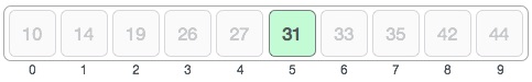
Let the given array be

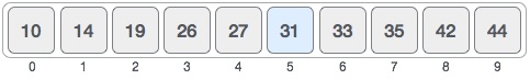
and the number to be searched be 31.

First determine the left and right ends of the array

left = 0 and right = n-1 (here n = 10, the size of array). Thus middle = left + (right - left) / 2 .

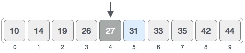
Now, compare the arr[mid] value with x (value to be found). If arr[mid] > x, then we can say x lies to the left of mid. Else if arr[mid] < x, then x lies to the right of mid, else if arr[mid] == x we have found our ans.

Here arr[mid] < 31, thus we change our left = mid+1 and mid = left + (right - left) / 2

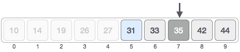
Here arr[mid] > 31, thus we change our right = mid-1 and mid = left + (right - left) / 2

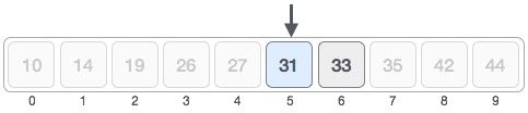
Finally arr[mid] = 31, thus the required pos is mid, where mid = 5

int binarySearch(int arr[],int n, int x){
    int left=0, right=n-1;
    while(left<right){
        int mid=left+(right-left)/2;
        if(arr[mid]>x){
            right=mid-1;
        }
        else if(arr[mid]<x){
            left=mid+1;
        }
        else if(arr[mid]==x){
            return mid;
        }
    }
    return -1; // if x is not present in the array
}

Time Complexity

As mentioned earlier, Binary Search is the fastest algorithm with the time complexity of O(log₂n).

As we keep dividing the array to half it's current size at each iteration, thus the size of the array decreases logarithmically.

At 1st iteration

length = n

At 2nd iteration

length = $ \frac{x}{2} $

At 3rd iteration

length = $\frac{x}{2}*\frac{1}{2} = \frac{x}{4}$

. . .

At k-th iteration

length = $ \frac{n}{2^{k-1}} $

So, maximum number of interations will be $ \log_2{n} $

Practice Probelms

Binary Search

Intresting Drink

Books

Know These

upper_ bound:

In-built C++ function, which takes an array or a vector and a value ( say x ) as input and returns a iterator that points to a value just greater than the provided value. ( works on a sorted array / vector ). If there are multiple such values, the one that makes first occurance is returned.

vector<int> v;
int x;
int pos = upper_bound( v.begin() , v.end(), x) - v.begin();

lower_bound:

In-built C++ function, which takes an array or a vector and a value ( say x ) as input and returns an iterator that points to the value not less than the provided value. ( works on a sorted array / vector ). If there are multiple such values, the one that makes first occurance is returned.

vector<int> v;
int x;
int pos = lower_bound( v.begin() , v.end() , x) - v.begin();

If no such value is available, both the functions return an iterator pointing to the end of the array / vector .

Binary Search VS Linear Search

As we can judge from the time complexities, Binary search is the go to method for a sorted array.

The GIF belows visualises Binary-Search and Linear-Search side by side on the same array. Hope, this gives you an idea of the algorithms efficiency.

Ternary Search

It is a divide-and-conquer algorithm, similar to binary search, only that we divide the array in three parts using mid1 and mid2, and the array should be sorted.

Problem Statement

Solution

Let the given array be

1 | 2 | 3 | 4 | 5 | 6 | 7 | 8 | 9 | 10

and the value to be searched be x = 6

First determine the left and right ends of the array

left = 0, right = 9 [n(size of array) - 1]

Thus, mid1 = left + ( right - left ) / 3, and

mid2 = mid1 + ( right - left ) / 3

left                         mid1                         mid2                          right
\/                               \/                                \/                                 \/
1    |    2    |    3    |    4    |    5    |    6    |    7    |    8    |    9    |    10

As, x > arr[mid1] and x < arr[mid2]

left = mid1 (4),
right = mid2 (7),
mid1 = 5,

mid2 = 6

                                left   mid1   mid2   right
                                  \/         \/        \/         \/
1    |    2    |    3    |    4    |    5    |    6    |    7    |    8    |    9    |    10

We see, arr[mid2] = x. Thus, required pos = mid2.

int ternarySearch(int arr[], int n,int l,int r int x){
    if(right > left){
        int mid1 = left + (right - left) / 3;
        int mid2 = mid1 + (right - left) / 3;
        // check if x is found
        if(arr[mid1] == x){
            retrun mid1;
        }
        if(arr[mid2] == x){
            retrun mid2;
        }
        if(x < arr[mid1]){
            // x lies between l and mid1
            return ternarySearch(arr, n, l, mid1-1, x);
        }
        else if(x > arr[mid2]){
            // x lies between mid2 nad r
            retrun ternarySearch(arr, n, mid2+1, r, x);
        }
        else{
            // x lies between mid1 and mid2
            return ternarySearch(arr, n, mid1+1, mid2-1, x);
        }
    }
    // x not found
    return -1;
}

Time Complexity

Ternary Search is faster than Binary Search, as it also works in logarithamic complexity but the base is 3, O(log₃n). But it is not as widely used as binary search.

As we keep dividing the array to one-third it's current size at each iteration, thus the size of the array decreases logarithmically.

At 1st iteration

length = n

At 2nd iteration

length = $ \frac{x}{3} $

At 3rd iteration

length = $\frac{x}{3}*\frac{1}{3} = \frac{x}{9}$

. . .

At k-th iteration

length = $ \frac{n}{3^{k-1}} $

So, maximum number of interations will be $ \log_3{n} $

Practice Problem

Weakness and Poorness

Race Time!

Devu and his Brother

This is JEE

Sorting Algorithms

A Sorting Algorithm is used to rearrange a given array or list elements according to a comparison operator on the elements. The comparison operator is used to decide the new order of element in the respective data structure.

Topics Covered

Bubble Sort

Example Problem

Given an array arr = [a1,a2,a3,a4,a5...,an] , we need to sort the array the array with the help of Bubble Sort algorithm.

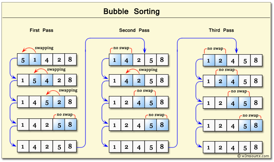
Discussion

Bubble Sort is one of the simplest sorting algorithms that repeatedly swaps the adjacent elements if they are in wrong order.

Illustration

Code for Bubble Sort


void bubbleSort(int arr[])
    {
        int n = arr.length;
        for (int i = 0; i < n-1; i++)
            for (int j = 0; j < n-i-1; j++)
                if (arr[j] > arr[j+1]) //if ordering is wrong
                {   int temp = arr[j]; //then swap a[j] and a[j+1]
                    arr[j] = arr[j+1];
                    arr[j+1] = temp;
                }
    }

Quick Sort

Example Problem

Given an array arr = [a1,a2,a3,a4,a5...,an] , we need to sort the array the array with the help of Quick Sort algorithm.

Discussion

So the basic idea behind Quick Sort is to take an element generally called the pivot and place it at such a place such that it is in it's sorted position.

Look at the following list of numbers:

10 36 15 23 56 12

Can you guess the number at the sorted position ? Yes it can be identified by just at glance , that is 10.

Now Let's take another example:

40 36 15 50 75 62 57

Now we can see that 50 is at it's sorted poition by just a glance. This is because all the elements before it is less than 50 and all elemnts after it is greater than 50.

So , the main idea is to select a pivot and place it to it's sorted position.

Working of the Algorithm

Let us take an example with the list of integers

50 70 60 90 40 80 10 20 30

Let us take the first element to be pivot that is 50.

Take two pointers i , j . Initially place i at the pivot i.e. index 0 and j at position n and keep a number (say infinite) at index n.

So, it looks like :

50 70 60 90 40 80 10 20 30 INT_MAX
i                          j

Now iterate i towards right and j towards left . Stop when arr[i]>pivot and arr[j]<=pivot . If i < j swap the values . Continue the process until i>j . Whwn this case arrives swap the pivot with arr[j].

Illustration

50 70 60 90 40 80 10 20 30 INT_MAX
   i                    j

// Here arr[i]>=50 and arr[j]<50 , so we swap them and move the pointers since i<j.

50 30 60 90 40 80 10 20 70 INT_MAX
      i              j

// Swapping again , and moving pointers.

50 30 20 90 40 80 10 60 70 INT_MAX
         i        j

// Swapping again , and moving pointers.

50 30 20 10 40 80 90 60 70 INT_MAX
            j  i

// Now we see j<i , so we stop the loop and swap arr[j] with pivot.

40 30 20 10 50 80 90 60 70 INT_MAX
            __

Now , we see that all elements before 50 are lesser than 50 and all elemnts after 50 are greater than 50.

Now apply this partitioning on both sides of 50 and hence, we will get our sorted array.

Code

Code For Partition

int partition(int a[],int l ,int h)
{
    int pivot = a[l]; // choosing left-most elemnt to be pivot
    int i=l,j=h;    // setting pointers i and j

    //looping through the process until we get j<i
    do{
        // iterating i until we get a number greater than pivot
        while(a[++i]<=pivot);

        // iterating j until we get a number greater than pivot
        while(a[--j]>pivot);

        //swapping arr[i] and arr[j]
        if(i<j){
            swap(a[i],a[j]);
        }
        
    }while(i<j);

    // swapping pivot
    swap(a[j],a[l]);

    //return partition point
    return j;
}

Code for Quick Sort.

void QuickSort(int a[],int l,int h)
{
    int j;
    if(l<h)
    {
        j=partition(a,l,h); // taking the partition point
        QuickSort(a,l,j);   // Sorting the left side
        QuickSort(a,j+1,h); // Sorting right side
    }
}

Time Complexity

Worst Case	Best Case	Average Case
O ( n² )	O ( nlog₂n )	O ( nlog₂n )

Worst Case : The worst case occurs when the partition process always picks greatest or smallest element as pivot. If we consider above partition strategy where first element is always picked as pivot, the worst case would occur when the array is already sorted in increasing or decreasing order.

Best Case: The best case occurs when the partition process always picks the middle element as pivot.

Other Resources : GFG Blog

Count Sort

Example Problem

Given an array arr = [a1,a2,a3,a4,a5...,an] , we need to sort the array with the help of Count Sort algorithm.

Discussion

Counting sort is a sorting technique based on keys between a specific range. It works by counting the number of objects having distinct key values. Then doing some arithmetic to calculate the position of each object in the output sequence.

Take a count array of size max_element + 1 and initialise the array with 0 . Now iterate through the initial array and for each element x increase the value of count array at index x by 1.

But this method won't work for negative integers .

So we take a count array of size max_element - min_element + 1 and initialize with 0. Now iterate through the initial array and for each element x increase the value of count array at index x - min_element by 1.

Now Iterate through the count array and if value at the index + min_element is greater than 0 keep on adding the index value to the array , and decrement the value of the index by 1.

Working of the Algorithm

Consider array = [1 , 3 , -5 , 3 , 4 , -2 , 0]

Here max_element = -5 and min_element = 4

So, Create an array of size (4 - (-5) + 1) = 10 and initialise with 0.

count_array = [ 0 , 0 , 0 , 0 , 0 , 0 , 0 , 0 , 0 , 0 ]
idx_values->    0   1   2   3   4   5   6   7   8   9

After the iteration , count array becomes ->

count_array = [ 1 , 0 , 0 , 1 , 0 , 1 , 1 , 0 , 2 , 1 ]
idx_values->    0   1   2   3   4   5   6   7   8   9

The Sorted Array becomes : [-5 , -2 , 0 , 1 , 3 , 3 , 4]

Code

Code For Count Sort

void CountSort(int a[],int n)
{
    int max_element = -INT_MAX , min_element = INT_MAX ;

    // for finding the max_element in the array
    for(int i=0;i<n;i++)
        max_element = max(max_element , a[i]);
    
    // for finding the min_element in the array
    for(int i=0;i<n;i++)
        min_element = min(min_element , a[i]);

    // initisalizing a count vector of size max_element - min_element + 1
    vector <int> count(max_element - min_element +1 , 0);

    // setting count vector according to the algorithm
    for(int i=0;i<n;i++)
        count[a[i] - min_element]++;
    
    // updating the actual array
    int j = 0,i=0;
    while(i<max_element - min_element +1)
    {
        if(count[i] == 0)
            i++;
        else
        {
            a[j] = min_element + i;
            count[i]--;
            j++;
        }
        
    }
}

Time Complexity

Time Complexity: O(n+k) where n is the number of elements in input array and k is the range of input.

Space Complexity: Algorithm takes extra space of O(k).

Important

Counting sort is efficient if the range of input data is not significantly greater than the number of objects to be sorted. Consider the situation where the input sequence is between range 1 to 10K and the data is 10, 5, 10K, 5K.

Other Resources : GFG Blog

Bucket Sort

Example Problem

Given an array arr = [a1,a2,a3,a4,a5...,an] , we need to sort the array with the help of Bucket Sort algorithm.

Discussion

Bucket Sort is a sorting technique that sorts the elements by first dividing the elements into several groups called buckets. The elements inside each bucket are sorted using any of the suitable sorting algorithms or recursively calling the same algorithm.

Working of the Algorithm

Several buckets are created. Each bucket is filled with a specific range of elements. The elements inside the bucket are sorted using any other algorithm. Finally, the elements of the bucket are gathered to get the sorted array.

The process of bucket sort can be understood as a scatter-gather approach. The elements are first scattered into buckets then the elements of buckets are sorted. Finally, the elements are gathered in order.

Bucket Sort

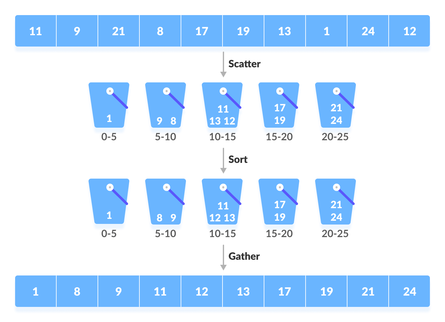
Illustration

Let's Sort an array of decimal numbers in th range 0 to 1.

Input array : 0.42 0.32 0.23 0.52 0.25 0.47 0.51

Create an array of size 10. Each slot of this array is used as a bucket for storing elements.

Insert elements into the buckets from the array. The elements are inserted according to the range of the bucket. And Sort them with a suitable sorting technique.

Representation of the buckets ->

|   |   | 0.23 |      | 0.42 | 0.51 |   |   |   |   |
| 0 | 0 | 0.25 | 0.32 | 0.47 | 0.52 | 0 | 0 | 0 | 0 |
  
  0   1    2      3      4       5    6   7   8   9

Traverse From Left to right and put the elements back into array in the same order.

Sorted Array : 0.23 0.25 0.32 0.42 0.47 0.51 0.52

Code

Code For Bucket Sort.

void BucketSort(double a[],int n)
{
    // creating vector array of size 10
    vector <double> bucket[10];

    // putting elements in respective bucket
    for(int i=0;i<n;i++)
        bucket[ int(10 * a[i]) ].push_back(a[i]);
    
    // sorting each bucket with quick sort
    for(int i=0;i<10;i++)
        sort(bucket[i].begin(),bucket[i].end());

    // picking from bucket and placing back to the array
    for(int i=0, j=0;i<10;i++)
    {
        for(auto x : bucket[i])
        {
            a[j] = x;
            j++;
        }
    }

    // clearing the each bucket
    for(int i=0;i<10;i++)
        bucket[i].clear();
}

Time Complexity

Worst Case Complexity : O ( n² )

When there are elements of close range in the array, they are likely to be placed in the same bucket. This may result in some buckets having more number of elements than others. It makes the complexity depend on the sorting algorithm used to sort the elements of the bucket.

The complexity becomes even worse when the elements are in reverse order. If insertion sort is used to sort elements of the bucket, then the time complexity becomes O ( n² ).

Best Case Complexity: O(n+k)

It occurs when the elements are uniformly distributed in the buckets with a nearly equal number of elements in each bucket. The complexity becomes even better if the elements inside the buckets are already sorted.

If insertion sort is used to sort elements of a bucket then the overall complexity in the best case will be linear ie. O(n+k). O(n) is the complexity for making the buckets and O(k) is the complexity for sorting the elements of the bucket using algorithms having linear time complexity at the best case.

Other Resources : GFG Blog

Heap Sort

Example Problem

Given an array arr = [a1,a2,a3,a4,a5...,an] , we need to sort the array with the help of Heap Sort algorithm.

Discussion

Heap sort is a comparison based sorting technique based on Binary Heap data structure. It is similar to selection sort where we first find the maximum element and place the maximum element at the end. We repeat the same process for the remaining elements.

A Binary Heap is a Complete Binary Tree where items are stored in a special order such that value in a parent node is greater(or smaller) than the values in its two children nodes. The former is called as max heap and the latter is called min-heap. The heap can be represented by a binary tree or array.

Here , we use array representation of complete binary tree. So for the index i the left child will be 2*i and the right child will be 2*i+1.

Working of the Algorithm

Heap Sort Algorithm for sorting in increasing order:

Build a max heap from the input data.
At this point, the largest item is stored at the root of the heap. Replace it with the last item of the heap followed by reducing the size of heap by 1. Finally, heapify the root of the tree.
Repeat step 2 while size of heap is greater than 1.

Algorithm for building max heap:

A single element is already in a heap.
When we add next elemnt , add it at the last of the array, so that it is a complete binary tree.
Now , the newly inserted element is a leaf element. So we compare the element with it's parent element (i/2) and if the inserted element is greater than it's parent we place the parent node at the leaf position . And we repeat this process , until we find the proper position for the newly inserted element.

Algorithm for deletion:

We can only delete a root element from the max heap.
So we swap the last element of the complete binary tree with the root element and bring the root element to it's proper position. In this process the size of max heap decreases by 1.

Illustration

Input data : 6 25 10 5 40

Now , as discussed above 6 that is the single element is already a heap.

Inserting 25 ->

          6        Applying Heap       25
         /        -------------->     /
        25                           6

Inserting 10 ->

         25        Applying Heap       25
        /  \      --------------->    /  \
       6    10                       6    10

Repeating the same process , the final heap is ->

                    40
                   /  \
                 25    10
                /  \ 
               5    6   

So the new array becomes : 40 25 10 5 6

We have build our max heap , now we keep on deleting the root element and keep on adding the element at the end of the array and put the last element of the heap to the node.

      6                                      25
     / \        Making it Heap again        /  \
   25   10       --------------->          6    10
   /                                      /
  5                                      5

So now the array becomes : 25 6 10 5 || 40 , where the elements before || is a heap.

Repeating the same process until the size of the heap becomes 1 , our array becomes : 5 6 10 25 40

Hence the array is sorted.

Code

Code For Insertion

void InsertHeap(int arr[],int n)
{
    // taking the newly inserted element as temp
    int temp = arr[n] , i = n;

    // finding correct position for temp
    while(i>1 && temp>arr[i/2])
    {
        arr[i] = arr[i/2];
        i/=2;
    }

    //placing the temp at the correct position
    arr[i] = temp;
}

Code for Deletion.

void DeleteHeap(int a[],int n)
{
    int i = 1;
    int j = i*2;

    // swapping the root and the last element
    swap(a[1],a[n]);

    // coverting the rest array into heap again
    while(j<n-1)
    {
        // comparing the left and right child for finding the greater one
        if(a[j+1]>a[j])
            j = j+1;

        // cehcking for the correct position
        if(a[i]<a[j])
        {
            swap(a[i],a[j]);
            i = j;
            j = j*2;
        }
        else
            break;
    }
}

Code for Heap Sort.

void HeapSort(int a[],int n)
{
    // making the max heap
    for(int i=2;i<n;i++)
        InsertHeap(a,i);
    
    // deleting the root and placing at last of the array
    for(int i=n;i>1;i--)
        DeleteHeap(a,i);
}

Time Complexity

Each Insertion algorithm takes O(logn) time and we insert n number of elements in the heap , so the total time complexity for insertion is O(nlogn).

Similarly , each Insertion algorithm takes O(logn) time and we delete n number of elements in the heap , so the total time complexity for deletion is O(nlogn).

So the total time complexity for heap sort is (nlogn).

Note

One thing to be noted is that , the time complexity of insertion algorithm can be reduced by using heapify. In heapify we check elemnts from last and see if the elemnt is greater than it's child element . If it is not then we apply heapify on the sub tree to make it a proper heap.

Code for Heapify

void heapify(int arr[], int n, int i)
{
    int largest = i; // Initialize largest as root
    int l = 2 * i + 1;
    int r = 2 * i + 2;
 
    // If left child is larger than root
    if (l < n && arr[l] > arr[largest])
        largest = l;
 
    // If right child is larger than largest so far
    if (r < n && arr[r] > arr[largest])
        largest = r;
 
    // If largest is not root
    if (largest != i) {
        swap(arr[i], arr[largest]);
 
        // Recursively heapify the affected sub-tree
        heapify(arr, n, largest);
    }
}

Code for Heap Sort

void heapSort(int arr[], int n)
{
    // Build heap (rearrange array)
    for (int i = n / 2 - 1; i >= 0; i--)
        heapify(arr, n, i);
 
    // One by one extract an element from heap
    for (int i = n - 1; i > 0; i--) {
        // Move current root to end
        swap(arr[0], arr[i]);
 
        // call max heapify on the reduced heap
        heapify(arr, i, 0);
    }
}

Above Code is from GFG Blog.

Application Problems

Radix Sort

Example Problem

Given an array arr = [a1,a2,a3,a4,a5...,an] , we need to sort the array the array with the help of Radix Sort algorithm.

Discussion

Since you are reading this , I assume that you have already gone through most of the comparison sorts that is Merge Sort , Quick Sort , etc . Problem with comparison based algorithm is that the lower bound complexity for them is nlogn. They cannot do better than that.

Counting Sort , Bin Bucket Sort can be used to tackle this problem , but problem with counting sort is that if the maximum number in the array is of the order n² , then the running time complexity would be of the order O(n²). Also the extra space required increases with the maximum number.

The idea of Radix Sort is to do digit by digit sort starting from least significant digit to most significant digit. Radix sort uses counting sort as a subroutine to sort.

Working of the Algorithm

Do following for each digit i where i varies from least significant digit to the most significant digit.

Sort input array using counting sort (or any stable sort) according to the i’th digit.
Update The array.

Illustration

Let us look at the following illustration :

23 20 15 5 61 301 17 33

Let's look at the one's position for each of the numbers.

23  20  15  5  61  301  17  33
 _   _   _  _   _    _   _   _

Sort them according to the marked digits. If there are same digits put them from left to right according to the array.

20  61  301  23  33  15  05  17
_   _    _   _   _   _   _   _

Sort them again according to Ten's place.

301  005  015  017  020  023  033  061
_    _    _    _    _    _    _    _

Sort them again according to Hundred's place.

005  015  017  020  023  033  061  301

We get the final sorted array.

5 15 17 20 23 33 61 301

Code

Code For Sorting according to digits

void digit_sort(int a[],int n,int exp)
{
    // declaring vector array of size 10. Since there are 10 digits.
    vector <int> arr[10];

    // pushing each number in their respective buckets.
    for(int i=0;i<n;i++){
        arr[ (a[i]/exp) % 10 ].push_back(a[i]);
    }

    int j = 0;

    // Updating the main array.
    for(int i=0;i<10;i++)
    {
        for(auto x:arr[i]){
            a[j] = x;
            j++;
        }
    }

    // deleting the extra space.
    for(int i=0;i<10;i++)
        arr[i].clear();
}

Code for Radix Sort.

void RadixSort(int a[],int n)
{
    // function for finding the max digit
    int m = max_digit(a,n);

    for(int i=1;i<=m;i++)
    {
        // digit_sort for each place
        digit_sort(a,n,int(pow(10,i-1)+0.5));
    }
}

Code for finding maximum number of digits.

int max_digit(int a[], int n)
{
    int res = 0;
    for(int i=0;i<n;i++)
    {
        int temp = a[i] , count = 0;
        while(temp)
        {
            temp/=10;
            count++;
        }
        res = max(res,count);
    }
    return res;
}

Time Complexity

What is the running time of Radix Sort?

Let there be d digits in input integers. Radix Sort takes O(d*(n+b)) time where b is the base for representing numbers, for example, for the decimal system, b is 10. What is the value of d? If k is the maximum possible value, then d would be O(logb(k)). So overall time complexity is O((n+b) * logb(k)). Which looks more than the time complexity of comparison-based sorting algorithms for a large k. Let us first limit k. Let k <= nc where c is a constant. In that case, the complexity becomes O(nLogb(n)). But it still doesn’t beat comparison-based sorting algorithms.

What if we make the value of b larger?.

What should be the value of b to make the time complexity linear? If we set b as n, we get the time complexity as O(n). In other words, we can sort an array of integers with a range from 1 to nc if the numbers are represented in base n (or every digit takes log2(n) bits).

Other Resources : GFG Blog

Insertion Sort

Example Problem

Given an array arr = [a1,a2,a3,a4,a5...,an] , we need to sort the array the array with the help of Insertion Sort algorithm.

Discussion

Look at the following list of numbers:

36 10 5 23 56 12

We scan the array from left to right. For every element in the array, we must ensure that the elements to the left are less than the current element( for sorting in ascending order) and the elements to the right have not yet been seen.

We take 2 pointers- i,j. We exchange arr[i] with each larger element to its left. At first, the pointer i is at position 0. So arr[0]=36 is at its correct position since there is there no element to its left.

We then increment the pointer ''i''. The pointer i now points to arr[1]=10. Now the element to the left of 10 is 36. We see that the element 10 is not in its correct position, since there is an element to the left(=36) which is greater than 10. So we exchange their positions. The present array is 10 36.

We increment the pointer to point at arr[2]=5. The element 5 is not at its correct position. So we exchange 5 with 36. The current array is 10 5 36. The element 5 is still not in its correct position as 10 is greater than 5. So we exchange 10 with 5. The current array becomes 5 10 36.

We continue this way.

Note: | marks the position of j.
When i=0:
36 | 10 5 23 56 12

When i=1:
36 10 | 5 23 56 12
//36 greater than 10. So we exchange.
10 | 36 5 23 56 12
//Go no further as there is no element to left.

When i=2:
10 36 5 | 23 56 12
//36 grrater than 5. So we exchange.
10 5 | 36 23 56 12
//10 greater than 5 . So we exchange.
5 | 10 36 23 56 12
//5 is at its correct position.

When i=3:
5 10 36 23 | 56 12
//We exchange 36 and 23 as 36>23.
5 10 23 | 36 56 12
//10<23. So we need not go any further.

When i=4:
5 10 23 36 56 | 12
//56 is larger than every element to the left. So no exchange needed.

When i=5:
5 10 23 36 56 12 |
//12 is smaller than 56. So we exchange.
5 10 23 36 12 | 56
//12 is smaller than 36. So we exchange.
5 10 23 12 | 36 56
//12 is smaller than 23. So exchange is needed.
5 10 12 | 23 36 56
//12 is greater than 10. Hence we stop.

At this position we stop since we have traversed through the entire array.

Code for the Algorithm

Code For Insertion Sort

public void sort(Comparable []a){
   for(int i=0;i<a.length;i++){
      for (int j = i; j > 0; j--){
         if (less(a[j], a[j-1]))//if element at j is less than the element at j-1
            exch(a, j, j-1);    //we exchange the two elements. 
         else break;
      }
   }

}

Shell Sort

Example Problem

Given an array arr = [a1,a2,a3,a4,a5...,an] , we need to sort the array the array with the help of Shell Sort algorithm.

Discussion

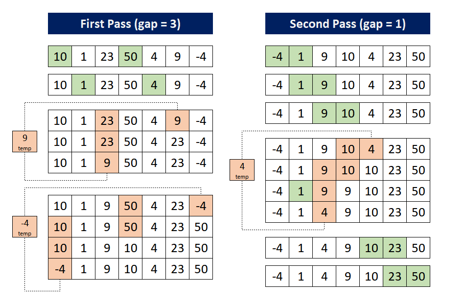
Shell Sort is an improvement in the Insertion sort algorithm. It can be observed that the insertion sort works extremely well on almost sorted array. Shell sort makes use of this. We make the array h-sorted for a large value of h using the technique of insertion sort. We then keep reducing the value of h until it becomes 1.

Note: An array is said to be h-sorted if all sublists of every h'th element is sorted.

Illustration:

Code for the Algorithm

Determining the value of h for h-sorting

while(h<n/3)h=3*h+1;

Code For Shell Sort

while(h>=1){
     for(int i=h;i<n;i++){
     //perform insertion sort for every h'th element
         for(int j=i;j>=h && less(a[j],a[j-h]);j-=h){
             exch(a,j,j-h);
         }
     }
     h=h/3;
 }

Resources

GeeksforGeeks

Merge Sort

Example Problem

Given an array arr = [a1,a2,a3,a4,a5...,an] , we need to sort the array the array with the help of Merge Sort algorithm.

Discussion

Merge sort is an application of the Divide and Conquer Principle.The basic approach is to:

Divide the array into two halves
Sort each half recursively
Merge the two halves

Code For Merge Sort

Merge Sort:

public static void mergesort(Comparable[] workplace,int lowerbound,int upperbound){
        if(lowerbound==upperbound){
            return;
        }
        else{
        int mid=(lowerbound+upperbound)/2;
        mergesort(workplace,lowerbound,mid);
        mergesort(workplace,mid+1,upperbound);
        merge(workplace,lowerbound,mid+1,upperbound);
        }
    }

Merging two sorted arrays:

public static void merge(Comparable[] workplace,int lowPtr,int highPtr,int upperbound)
    {
        int low=lowPtr;
        int mid=highPtr-1;
        int j=0;
        int n=upperbound-low+1;
        while(low<=mid && highPtr<=upperbound){
           if(theArray[low].compareTo(theArray[highPtr])<0){
               workplace[j++]=theArray[low++];
            }else{
                workplace[j++]=theArray[highPtr++];
            }
        }
        
        while(low<=mid){
            workplace[j++]=theArray[low++];
        }
        
        while(highPtr<=upperbound){
            workplace[j++]=theArray[highPtr++];
        }
        
        for(j=0;j<n;j++){
            theArray[lowPtr+j]=workplace[j];
        }
    }

Time Complexity:

Time complexity of Merge Sort is O(n*Log n) in all the 3 cases (worst, average and best) as merge sort always divides the array in two halves and takes linear time to merge two halves. It requires equal amount of additional space as the unsorted array.

Resources:

GeeksforGeeks

Selection Sort

Example Problem

Given an array arr = [a1,a2,a3,a4,a5...,an] , we need to sort the array the array with the help of Selection Sort algorithm.

Discussion

Selection sort is a simple sorting algorithm where we divide an array into two parts- sorted and unsorted. Initially the sorted part is empty. We find the smallest element of the unsorted part. Then we swap it with the leftmost element of the unsorted part. The leftmost element then becomes a member of the sorted part.

selection

Code For Selection Sort

public static void sort(Comparable a[])
    {
        // initialise instance variables
        for(int i=0;i<a.length;i++){
            int min=i;
            for(int j=i+1;j<a.length;j++){
                if(less(a[j],a[min])){//if a[j] less than min
                    min=j;             //then update position of min
                }
            }
            exch(a,i,min);//swap the i-th element with the minimum element
        }
    }

Resources:

HackerEarth

What is Backtracking?

Backtracking is an algorithmic-technique for solving problems recursively by trying to build a solution incrementally, one piece at a time, and abandons a candidate (or "backtracks") as soon as it determines that the candidate cannot possibly result in a valid solution.

Where is it used?

Usually in constraint satisfaction problems. Backtracking is useful while solving certain NP-complete problems where the theoretical upperbound is as bad as N! or 2 ^ N or even N ^ N.

N Queens

Typical backtracking recursive function

Explanation

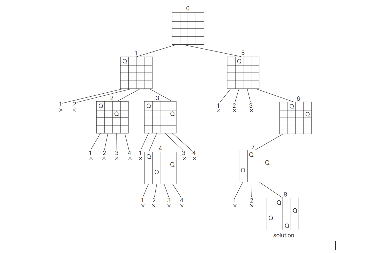
The backtracking algorithm uses recursion and so can be represented as a tree structure where each node differs from its parent by a single extension step. The leaves of the tree are nodes where there is no more extension possible (either the problem is solved, or there are no valid candidates satisfying the contraints at the next extension).

The search tree is traversed from root down in depth-first order. At each node, we check if the node leads us to the path giving us a complete valid solution. If not, then the whole subtree rooted at that node is skipped, or pruned.

If the node itself is a valid solution (in which case it would be the leaf node), boolean value True is returned, indicating the solution has been found and we do not need to search any longer.

If a node lies on the path to the solution, then we return with boolean value True. This can be determined if the recursive call to its subtree returns True or not.

The distance of a node from the root determines how many values have been filled in yet.

Pseudocode


def solve_backtrack():
    if is_solved(): // base case: solution has been found
        return True

    for candidate in candidates:
        if not is_feasible(candidate): // if candidate is not a valid choice
            continue

        accept(candidate) // use candidate for the current instance
        if solve_backtrack(): // recursive call
            return True // if problem solved, return True
        reject(candidate) // problem not solved, remove candidate used and continue in loop

    return False // solution does not exist

Common Backtracking Problems

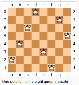
N Queens

Problem Statement:

In a chess game, a Queen can move along 3 axes - horizontal, vertical and diagonal. In this problem, we have an N x N chess board.

Place N Queens on this board in such a way that no two Queens can kill each other (no Queen can reach the position of another Queen in just one move).

N Queens

Sudoku

Problem Statement:

A sudoku grid is usually a 9 x 9 grid, with some blocks containing a few numbers initially. These numbers fall in the range 1 to 9. A sudoku grid is further divided into 9 3 x 3 subgrids.

We need to fill all the blocks in the grid with numbers from 1 to 9 only, while keeping the following constraints in mind:

Each row has only one occurrence of every number from 1 to 9
Each column has only one occurrence of every number from 1 to 9
Each subgrid has only one occurrence of every number from 1 to 9

A valid sudoku puzzle has a unique solution. However, puzzles with not enough initial values may have more than one valid solution - but these would not be valid sudoku puzzles.

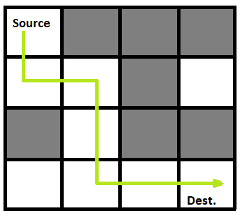
Maze Solver

Problem Statement:

Given a maze, a starting point and a finishing point, write a backtracking algorithm that will find a path from the starting point to the finishing point.

Maze Solver

String Permutation

Problem Statement:

Given a string, find all possible permutations that can be generated from it.

Example:

ABC

ACB

BAC

BCA

CAB

CBA

M Colouring

Problem Statement:

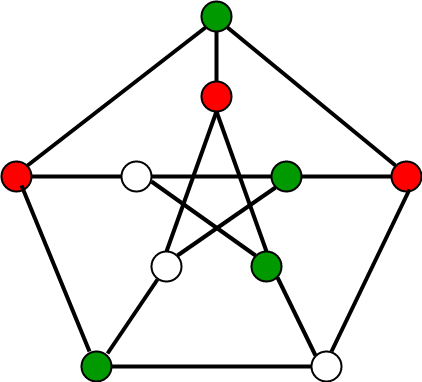
Given a graph, find a way to colour every node such that no two connected nodes (nodes which share an edge) are coloured the same and minimum possible number of colours are used.

On a side-but-related note, one might be interested to check out the four colour theorem, proved in 1976.

M Colouring Graph

Persistent Data Structure

In normal DS when we change or update a particular value the entire DS gets changed. Consider an array arr = [1, 2, 3, 4, 4], now if we want to update arr[2] to 6 it will become [1, 2, 6, 4, 4]. This final array now lost its pervious state. But in case of Persistent DS it will preserve it's previous states as well.

Persistent Datastructure preserves all versions of itself

Every update to the data structure creates a new version
Update(version, <value>): returns a new version

Types of Persistence

1. Parital Persistence

Query any versions of the DS
Update only the latest version of DS

Let's say we have a series of versions as follows (in the form of Linked List):

v1 -> v2 -> v3

Now if we want to make some changes we can only do that to the v3, so after this update we will have

v1 -> v2 -> v3 -> v4

Hence, all the versions will always be linearly ordered (due to the additional constraint)

2. Full Persistence

Query any versions of the DS (typical of any persistence)
Update any version of the DS

Let's say initially you only one version v1, and then you make an update you get

v1 -> v2

Now you apply another update but again to v1 (this was not possible in partial persistence) here it will branch off as show below

        v1
       /  \ 
     v2    v3

Again if we update v3 we will get:-

Hence, in full persistence the versions will form a tree.

A DS that supports full persistence will always support partial persistence.

Persistent segment tree

Example problem :

We have an array a1, a2, ..., an and at first q update queries and then u ask queries which you have to answer online. Each update query gives you numbers p and v and asks you to increase ap by v. Each ask query, gives you three numbers i and x and y and asks you to print the value of ax + ax + 1 + ... + ay after performing i - th query.

Solution

Each update query, changes the value of O(log(n)) nodes in the segment tree, so you should keep rest of nodes (not containing p) and create log(n) new nodes. Totally, you need to have q.log(n) nodes. So, you can not use normal segment's indexing, you should keep the index of children in the arrays L and R.

If you update a node, you should assign a new index to its interval (for i - th query).

You should keep an array root[q] which gives you the index of the interval of the root ( [0, n) ) after performing each query and a number ir = 0 which is its index in the initial segment tree (ans of course, an array s[MAXNODES] which is the sum of elements in that node). Also you should have a NEXT_FREE_INDEX = 1 which is always the next free index for a node.

First of all, you need to build the initial segment tree :

(In these codes, all arrays and queries are 0-based)

void build(int id = ir,int l = 0,int r = n){
	if(r - l < 2){
		s[id] = a[l];
		return ;
	}
	int mid = (l+r)/2;
	L[id] = NEXT_FREE_INDEX ++;
	R[id] = NEXT_FREE_INDEX ++;
	build(L[id], l, mid);
	build(R[id], mid, r);
	s[id] = s[L[id]] + s[R[id]];
}

(So, we should call build() )

Update function : (its return value, is the index of the interval in the new version of segment tree and id is the index of old one)

int upd(int p, int v,int id,int l = 0,int r = n){
	int ID =  NEXT_FREE_INDEX ++; // index of the node in new version of segment tree
	if(r - l < 2){
		s[ID] = (a[p] += v);
		return ID;
	}
	int mid = (l+r)/2;
	L[ID] = L[id], R[ID] = R[id]; // in case of not updating the interval of left child or right child
	if(p < mid)
		L[ID] = upd(p, v, L[ID], l, mid);
	else
		R[ID] = upd(p, v, R[ID], mid, r);
	return ID;
}

(For the first query (with index 0) we should run root[0] = upd(p, v, ir) and for the rest of them, for j - th query se should run root[j] = upd(p, v, root[j - 1]) )

Function for ask queries :

int sum(int x,int y,int id,int l = 0,int r = n){
	if(x >= r or l >= y)	return 0;
	if(x <= l && r <= y)	return s[id];
	int mid = (l+r)/2;
	return sum(x, y, L[id], l, mid) +
	       sum(x, y, R[id], mid, r);
}

(So, we should print the value of sum(x, y, root[i]) )

Source: CF Blog

Tree

We can define Tree as a connected undirected graph with no cycles .

There are some more ways we can define Tree . Here are some equivalent definitions :

connected undirected graph with N nodes and N-1 edges.
connected undirected graph with only unique paths i.e there is one and only path from one node to another.
connected undirected graph where if you remove 1 edge it no longer remains connected.

Tree Algorithms :

Diameter of a tree

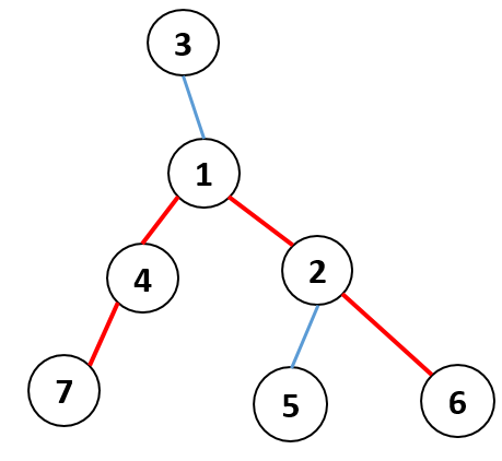
The Diameter of tree is the maximum length between two nodes. For example :
Consider the following tree of 7 nodes

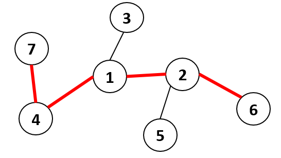
Here, Diameter = 4 .

Algorithm

First, root the tree arbitarily.

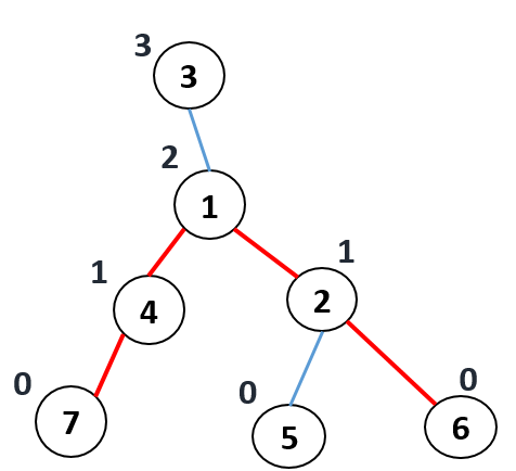
For each node, we calculate toLeaf(node) which denotes maximum length of a path from the node to any leaf.

if node is leaf :
    toLeaf[node] = 0
else
    toLeaf[node] = 1 + max(toLeaf[child]) | for all child of node

We can use DFS to calculate toLeaf(node).

vector<int> toLeaf(n+1, 0); // n is no. of nodes
void dfs(int node){
    visited[node] = true;
    for(int child : tree[node]){
        if(visited[child])
            continue;
        dfs(child);
        toLeaf[node] = max(toLeaf[node], 1 + toLeaf[child]);
    }
}

Now calculate path_length(node) which denotes maximum length of a path whose highest point is node.

if node is leaf :
    path_length[node] = 0
else if node has only 1 child :
    path_length[node] = toLeaf[child] + 1
else
    Take two distinct child a,b such that (toLeaf[a] + toLeaf[b]) is maximum, then
    path_length[node] = (toLeaf[a] + 1) + (toLeaf[b] + 1)

Here is the implementation .

vector<int> toLeaf(n+1, 0), path_length(n+1, 0);
void dfs(int node){
    visited[node] = true;
    vector<int> length = {-1}; // allows us to handle the cases when node has less than 2 children
    for(int child : tree[node]){
        if(visited[child])
            continue;
        dfs(child);
        toLeaf[node] = max(toLeaf[node], 1 + toLeaf[child]); 
        length.push_back(toLeaf[child]);
    }
    int s = length.size(), m = min((int)length.size(),2);
    for(int i = 0; i < m; i++){
        for(int j = i+1; j < s; j++){
            if(length[i] < length[j])
                swap(length[i], length[j]);
        }
        path_length[node] += length[i] + 1;
    }   
}

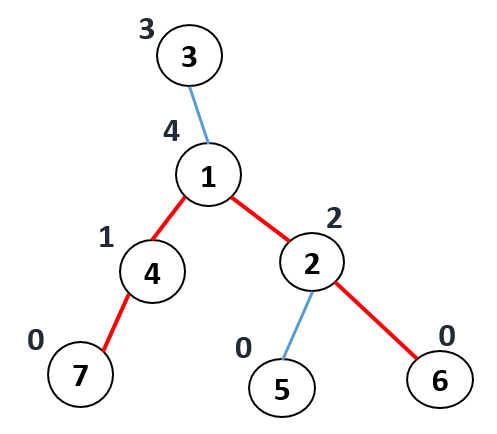
Finally, Diameter = maximum of all lengths in path_length. Therefore here, Diameter = 4.

Problems

Tree Diameter

Reference

Competitive Programmer's Handbook by Antii Laaksonen.

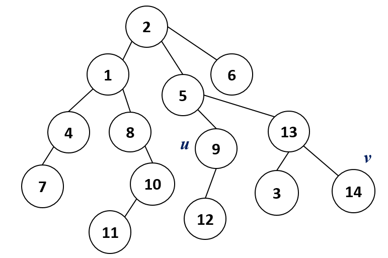
Lowest Common Ancestor

Given a rooted tree $T$ of $n$ nodes. The ancestors of a $node\ u$ are all the nodes in the path from $node\ u$ to $root$ (excluding $u$). Now Let's see how we can find $LCA$ of two $node\ u$ and $v$.

Algorithm $1$ : $O(n)$

climb up from the deeper $node$ such that $depth[u] == depth[v]$.
Now climb up from both the node until $u == v$.

Implementation :

int LCA(int u, int v){
    if(depth[u] > depth[v])
        swap(u, v);
    int h = depth[v] - depth[u];
    for(int i = 0; i < h; i++) // lifting v up to the same level as u
        v = parent[v];
    
    while(u != v){ // climbing up egde by egde from u and v
        u = parent[u];
        v = parent[v];
    }
    return u;
}

Here, as we are climbing edge by egde, hence in worst case it will take $O(n)$ time to compute LCA.

Algorithm $2$ : $O(logn)$

Instead of climbing edge by edge, we can make higher jumps from the node : say, from $node\ u$ to $2^i$ distant ancestor of $u$. We need to precompute $ancestor[n][k]$ : such that, $ancestor[i][j]$ will store $2^j$ distant ancestor of $node\ i$.

$n$ = no. of nodes if $2^k > n$, then we jump off the tree. Hence $ k = 1 + log_2(n) $

We know, $2^j = 2^{j-1} + 2^{j-1}$ therefore, $ancestor[i][j] = ancestor[\ ancestor[i][j-1]\ ][j-1]$ Note : $parent[root] = -1$; $ancestor[i][0]$ is simply the parent of $node\ i$.

// Computing ancestor table
int k = 1 + log2(n);
vector<vector<int>> ancestor(n+1, vector<int> (k));

for(int i = 1; i <= n; i++){
    ancestor[i][0] = parent[i];
}

for(int i = 1; i <= n; i++){
    for(int j = 1; j < k; j++){
        if(ancestor[i][j-1] != -1) // we didn't jump off the tree
            ancestor[i][j] = ancestor[ ancestor[i][j-1] ][j-1]
        else
            ancestor[i][j] = -1
    }
}

Binary Lifting :

Now say, we need to make a jump of height $h = 45$ from a $node\ u$. $h = 45 = (101101)_2 = (2^5 + 2^3 + 2^2 + 2^0) jumps$.
we can implement this jump as following :

int jump(int u, int h){
    for(int i = 0; h && u != -1;i++){
        if(h & 1)
            u = ancestor[u][i];
        h = h >> 1;
    }
    return u;
}

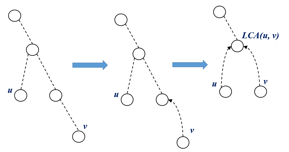
Computing LCA :

Using the $Binary\ Lifting$ technique, make jump of a $height = depth[v] - depth[u]$ from the deeper $node\ v$.

if $u == v$ already then $return\ u$.

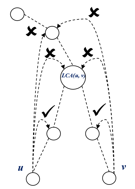
from $node\ u$ and $node\ v$, make jump as high as possible such that $ancestor[u][jump]\ != ancestor[v][jump]$, then eventually we will reach a node, $parent[u] = parent[v] = LCA(u, v)$

thus $return\ parent[u]$.

Implementation :

int LCA(int u, int v){
    if(depth[u] > depth[v])
        swap(u, v);
    v = jump(v, depth[v] - depth[u]);
    if(u == v)
        return u;
    
    int h = 1 + log2(depth[u]);
    for(int i = h-1; i >= 0; i--){
        if(ancestor[u][i] != -1 && ancestor[u][i] != ancestor[v][i]){
            u = ancestor[u][i];
            v = ancestor[v][i];
        }
    }
    return parent[u];
}

Problems

Reference

String Processing

A string is nothing but a sequence of symbols or characters. Sometimes, we come across problems where a string is given and the task is to search for a given pattern in that string. The straightforward method is to check by traversing the string index by index and searching for the pattern. But the process becomes slow when the length of the string increases. So, in this case hashing algorithms prove to be very useful. The topics covered are :

String Hashing

We need this to compare the strings. Idea is to convert each string to integer and compare those instead of the actual strings which is O(1) operation. The conversion is done by a Hash-Function and the integer obtained corresponding to the string is called hash of the string. A widely used function is polynomial rolling hash function :

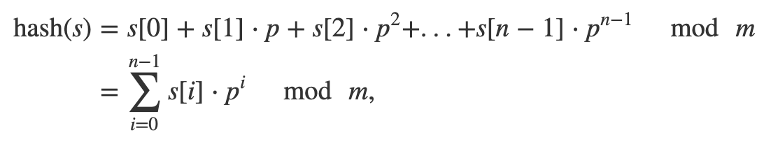
where p and m are some chosen, positive numbers. p is a prime approximately equal to the number of characters in the input alphabet and m is a large number. Here, it is m=10^9 + 9.

The number of possible characters is higher and pattern length can be large. So the numeric values cannot be practically stored as an integer. Therefore, the numeric value is calculated using modular arithmetic to make sure that the hash values can be stored in an integer variable.

Implementation

    long long compute_hash(string  const& s)
     { 
       const  int p = 31; 
       const  int m = 1e9 + 9;
       long  long hash_value = 0; 
       long  long p_pow = 1;
       for (char c : s) 
       {
         hash_value = (hash_value + (c - 'a' + 1) * p_pow)%m; 
         p_pow = (p_pow * p) % m;
       } 
       return hash_value; 
     }

Two strings with equal hashes need not be equal. There are possibilities of collision which can be resolved by simply calculating hashes using two different values of p and m which reduces the probability of collision.

Examples Of Uses

Find all the duplicate strings from a given list of strings
Find the number of different substrings in a string

Practice Problems

References

CP-Algorithms

Rabin-Karp Algorithm

This is one of the applications of String hashing.

Given two strings - a pattern s and a text t, determine if the pattern appears in the text and if it does, enumerate all its occurrences in O(|s|+|t|) time.

Algorithm : First the hash for the pattern s is calculated and then hash of all the substrings of text t of the same length as |s| is calculated. Now comparison between pattern and substring can be done in constant time.

Implementation

    vector<int> rabin_karp(string  const& s, string  const& t) 
    {
        const  int p = 31; 
        const  int m = 1e9 + 9;
        int S = s.size(), T = t.size();
        vector<long long> p_pow(max(S, T));
        p_pow[0] = 1; 
        for (int i = 1; i < (int)p_pow.size(); i++)
            p_pow[i] = (p_pow[i-1] * p) % m;
        vector<long long> h(T + 1, 0); 
        for (int i = 0; i < T; i++) 
            h[i+1] = (h[i] + (t[i] - 'a' + 1) * p_pow[i]) % m; 
        long  long h_s = 0; 
        for (int i = 0;i < S; i++) 
            h_s = (h_s + (s[i] - 'a' + 1) * p_pow[i]) % m;
        vector<int> occurences; 
        for (int i = 0; i + S - 1 < T; i++) 
        { 
            long  long cur_h = (h[i+S] + m - h[i]) % m;
            if (cur_h == h_s * p_pow[i] % m) 
            occurences.push_back(i); 
        } 
        return occurences; 
    }

Problems for Practice

References

CP-Algorithms

Machine Learning Algorithms

These are the engines of Machine Learning.

Topics Covered

Regression

These are the used to predict a continuous value.

Topics Covered

Linear Regression
- Linear Regression using Scikit-Learn
- Linear Regression using Matrix Multiplication
  - One Variable Linear Regression
  - Multiple Variable Linear Regression

Linear Regression

Linear Regression is a Supervised Machine Learning Method by which we find corelation between two or more than two variables, and then use it to predict the dependant variable, given independent variables.

Topics Covered

Linear Regression

Linear regression is perhaps one among the foremost necessary and wide used regression techniques. It’s among the only regression ways. one among its main blessings is that the simple deciphering results.

Problem Formulation

When implementing regression toward the mean of some variable quantity variable quantity the set of freelance variables 𝐱 = (𝑥₁, …, 𝑥ᵣ), wherever wherever is that the variety of predictors, you assume a linear relationship between 𝑦 and 𝐱: 𝑦 = 𝛽₀ + 𝛽₁𝑥₁ + ⋯ + 𝛽ᵣ𝑥ᵣ + 𝜀. This equation is that the regression of y on x. 𝛽₀, 𝛽₁, …, 𝛽ᵣ area unit the regression coefficients, and 𝜀 is that the random error.

Linear regression calculates the estimators of the regression coefficients or just the expected weights, denoted with 𝑏₀, 𝑏₁, …, 𝑏ᵣ. They outline the calculable regression operate 𝑓(𝐱) = 𝑏₀ + 𝑏₁𝑥₁ + ⋯ + 𝑏ᵣ𝑥ᵣ. This operate ought to capture the dependencies between the inputs and output sufficiently well.

The calculable or expected response, 𝑓(𝐱ᵢ), for every for every = one, …, 𝑛, ought to be as shut as potential to the corresponding actual response 𝑦ᵢ. The variations variations - 𝑓(𝐱ᵢ) for all observations 𝑖 = one, …, 𝑛, area unit known as the residuals. Regression is regarding deciding the most effective expected weights, that's the weights adore the littlest residuals.

To get the most effective weights, you always minimize the add of square residuals (SSR) for all observations 𝑖 = one, …, 𝑛: SSR = Σᵢ(𝑦ᵢ - 𝑓(𝐱ᵢ))². This approach is named the tactic of normal statistical procedure.

Regression Performance

The variation of actual responses 𝑦ᵢ, 𝑖 = 1, …, 𝑛, happens partially thanks to the dependence on the predictors 𝐱ᵢ. However, there's additionally a further inherent variance of the output.

The constant of determination, denoted as 𝑅², tells you which of them quantity of variation in 𝑦 will be explained by the dependence on 𝐱 mistreatment the actual regression model. Larger 𝑅² indicates a better fit and means that the model can better explain the variation of the output with different inputs.

The value 𝑅² = 1 corresponds to SSR = 0, that is to the perfect fit since the values of predicted and actual responses fit completely to each other.

Implementing Linear Regression in Python

It’s time to start implementing linear regression in Python. Basically, all you should do is apply the proper packages and their functions and classes.

Python Packages for Linear Regression

The package NumPy is a fundamental Python scientific package that allows many high-performance operations on single- and multi-dimensional arrays. It also offers many mathematical routines. Of course, it’s open source.

If you’re not familiar with NumPy, you can use the official NumPy User Guide .

The package scikit-learn is a widely used Python library for machine learning, built on top of NumPy and some other packages. It provides the means for preprocessing data, reducing dimensionality, implementing regression, classification, clustering, and more. Like NumPy, scikit-learn is also open source.

You can check the page Generalized Linear Models on the scikit-learn web site to learn more about linear models and get deeper insight into how this package works.

If you want to implement linear regression and need the functionality beyond the scope of scikit-learn, you should consider statsmodels. It’s a powerful Python package for the estimation of statistical models, performing tests, and more. It’s open source as well.

You can find more information on statsmodels on its official web site.

Simple Linear Regression With scikit-learn

Let’s start with the simplest case, which is simple linear regression.

There are five basic steps when you’re implementing linear regression:

Import the packages and classes you need.
Provide data to work with and eventually do appropriate transformations.
Create a regression model and fit it with existing data.
Check the results of model fitting to know whether the model is satisfactory.
Apply the model for predictions.

These steps are more or less general for most of the regression approaches and implementations.

Step 1: Import packages and classes

The first step is to import the package numpy and the class LinearRegression from sklearn.linear_model:

import numpy as np
from sklearn.linear_model import LinearRegression

Now, you have all the functionalities you need to implement linear regression.

The fundamental data type of NumPy is the array type called numpy.ndarray. The rest of this article uses the term array to refer to instances of the type numpy.ndarray.

The class sklearn.linear_model.LinearRegression will be used to perform linear and polynomial regression and make predictions accordingly.

Step 2: Provide data The second step is defining data to work with. The inputs (regressors, 𝑥) and output (predictor, 𝑦) should be arrays (the instances of the class numpy.ndarray) or similar objects. This is the simplest way of providing data for regression:

x = np.array([5, 15, 25, 35, 45, 55]).reshape((-1, 1))
y = np.array([5, 20, 14, 32, 22, 38])

Now, you have two arrays: the input x and output y. You should call .reshape() on x because this array is required to be two-dimensional, or to be more precise, to have one column and as many rows as necessary. That’s exactly what the argument (-1, 1) of .reshape() specifies.

This is how x and y look now:

>>> print(x)
[[ 5]
 [15]
 [25]
 [35]
 [45]
 [55]]
>>> print(y)
[ 5 20 14 32 22 38]

As you can see, x has two dimensions, and x.shape is (6, 1), while y has a single dimension, and y.shape is (6,).

Step 3: Create a model and fit it The next step is to create a linear regression model and fit it using the existing data.

Let’s create an instance of the class LinearRegression, which will represent the regression model:

model = LinearRegression()

This statement creates the variable model as the instance of LinearRegression. You can provide several optional parameters to LinearRegression:

fit_intercept is a Boolean (True by default) that decides whether to calculate the intercept 𝑏₀ (True) or consider it equal to zero (False).
normalize is a Boolean (False by default) that decides whether to normalize the input variables (True) or not (False).
copy_X is a Boolean (True by default) that decides whether to copy (True) or overwrite the input variables (False).
n_jobs is an integer or None (default) and represents the number of jobs used in parallel computation. None usually means one job and -1 to use all processors.

This example uses the default values of all parameters.

It’s time to start using the model. First, you need to call .fit() on model:

model.fit(x, y)

With .fit(), you calculate the optimal values of the weights 𝑏₀ and 𝑏₁, using the existing input and output (x and y) as the arguments. In other words, .fit() fits the model. It returns self, which is the variable model itself. That’s why you can replace the last two statements with this one:

model = LinearRegression().fit(x, y)

This statement does the same thing as the previous two. It’s just shorter.

Step 4: Get results

Once you have your model fitted, you can get the results to check whether the model works satisfactorily and interpret it.

You can obtain the coefficient of determination (𝑅²) with .score() called on model:

>>> r_sq = model.score(x, y)
>>> print('coefficient of determination:', r_sq)
coefficient of determination: 0.715875613747954

When you’re applying .score(), the arguments are also the predictor x and regressor y, and the return value is 𝑅².

The attributes of model are .intercept*, which represents the coefficient, 𝑏₀ and .coef*, which represents 𝑏₁:

>>> print('intercept:', model.intercept_)
intercept: 5.633333333333329
>>> print('slope:', model.coef_)
slope: [0.54]

The code above illustrates how to get 𝑏₀ and 𝑏₁. You can notice that .intercept* is a scalar, while .coef* is an array.

The value 𝑏₀ = 5.63 (approximately) illustrates that your model predicts the response 5.63 when 𝑥 is zero. The value 𝑏₁ = 0.54 means that the predicted response rises by 0.54 when 𝑥 is increased by one.

You should notice that you can provide y as a two-dimensional array as well. In this case, you’ll get a similar result. This is how it might look:

>>> new_model = LinearRegression().fit(x, y.reshape((-1, 1)))
>>> print('intercept:', new_model.intercept_)
intercept: [5.63333333]
>>> print('slope:', new_model.coef_)
slope: [[0.54]]

As you can see, this example is very similar to the previous one, but in this case, .intercept* is a one-dimensional array with the single element 𝑏₀, and .coef* is a two-dimensional array with the single element 𝑏₁.

Step 5: Predict response

Once there is a satisfactory model, you can use it for predictions with either existing or new data.

To obtain the predicted response, use .predict():

>>> y_pred = model.predict(x)
>>> print('predicted response:', y_pred, sep='\n')
predicted response:
[ 8.33333333 13.73333333 19.13333333 24.53333333 29.93333333 35.33333333]

When applying .predict(), you pass the regressor as the argument and get the corresponding predicted response.

This is a nearly identical way to predict the response:

>>> y_pred = model.intercept_ + model.coef_ * x
>>> print('predicted response:', y_pred, sep='\n')
predicted response:
[[ 8.33333333]
 [13.73333333]
 [19.13333333]
 [24.53333333]
 [29.93333333]
 [35.33333333]]

In this case, you multiply each element of x with model.coef* and add model.intercept* to the product.

The output here differs from the previous example only in dimensions. The predicted response is now a two-dimensional array, while in the previous case, it had one dimension.

If you reduce the number of dimensions of x to one, these two approaches will yield the same result. You can do this by replacing x with x.reshape(-1), x.flatten(), or x.ravel() when multiplying it with model.coef_.

In practice, regression models are often applied for forecasts. This means that you can use fitted models to calculate the outputs based on some other, new inputs:

>>> x_new = np.arange(5).reshape((-1, 1))
>>> print(x_new)
[[0]
 [1]
 [2]
 [3]
 [4]]
>>> y_new = model.predict(x_new)
>>> print(y_new)
[5.63333333 6.17333333 6.71333333 7.25333333 7.79333333]

Here .predict() is applied to the new regressor x_new and yields the response y_new. This example conveniently uses arange() from numpy to generate an array with the elements from 0 (inclusive) to 5 (exclusive), that is 0, 1, 2, 3, and 4.

You can find more information about LinearRegression on the official documentation page.

Multiple Linear Regression With scikit-learn

You can implement multiple linear regression following the same steps as you would for simple regression.

Steps 1 and 2: Import packages and classes, and provide data

First, you import numpy and sklearn.linear_model.LinearRegression and provide known inputs and output:

import numpy as np
from sklearn.linear_model import LinearRegression

x = [[0, 1], [5, 1], [15, 2], [25, 5], [35, 11], [45, 15], [55, 34], [60, 35]]
y = [4, 5, 20, 14, 32, 22, 38, 43]
x, y = np.array(x), np.array(y)

That’s a simple way to define the input x and output y. You can print x and y to see how they look now:

>>> print(x)
[[ 0  1]
 [ 5  1]
 [15  2]
 [25  5]
 [35 11]
 [45 15]
 [55 34]
 [60 35]]
>>> print(y)
[ 4  5 20 14 32 22 38 43]

In multiple linear regression, x is a two-dimensional array with at least two columns, while y is usually a one-dimensional array. This is a simple example of multiple linear regression, and x has exactly two columns.

Step 3: Create a model and fit it

The next step is to create the regression model as an instance of LinearRegression and fit it with .fit():

model = LinearRegression().fit(x, y)

The result of this statement is the variable model referring to the object of type LinearRegression. It represents the regression model fitted with existing data.

Step 4: Get results

You can obtain the properties of the model the same way as in the case of simple linear regression:

>>> r_sq = model.score(x, y)
>>> print('coefficient of determination:', r_sq)
coefficient of determination: 0.8615939258756776
>>> print('intercept:', model.intercept_)
intercept: 5.52257927519819
>>> print('slope:', model.coef_)
slope: [0.44706965 0.25502548]

You obtain the value of 𝑅² using .score() and the values of the estimators of regression coefficients with .intercept* and .coef*. Again, .intercept* holds the bias 𝑏₀, while now .coef* is an array containing 𝑏₁ and 𝑏₂ respectively.

In this example, the intercept is approximately 5.52, and this is the value of the predicted response when 𝑥₁ = 𝑥₂ = 0. The increase of 𝑥₁ by 1 yields the rise of the predicted response by 0.45. Similarly, when 𝑥₂ grows by 1, the response rises by 0.26.

Step 5: Predict response

Predictions also work the same way as in the case of simple linear regression:

>>> y_pred = model.predict(x)
>>> print('predicted response:', y_pred, sep='\n')
predicted response:
[ 5.77760476  8.012953   12.73867497 17.9744479  23.97529728 29.4660957
 38.78227633 41.27265006]

The predicted response is obtained with .predict(), which is very similar to the following:

>>> y_pred = model.intercept_ + np.sum(model.coef_ * x, axis=1)
>>> print('predicted response:', y_pred, sep='\n')
predicted response:
[ 5.77760476  8.012953   12.73867497 17.9744479  23.97529728 29.4660957
 38.78227633 41.27265006]

You can predict the output values by multiplying each column of the input with the appropriate weight, summing the results and adding the intercept to the sum.

You can apply this model to new data as well:

>>> x_new = np.arange(10).reshape((-1, 2))
>>> print(x_new)
[[0 1]
 [2 3]
 [4 5]
 [6 7]
 [8 9]]
>>> y_new = model.predict(x_new)
>>> print(y_new)
[ 5.77760476  7.18179502  8.58598528  9.99017554 11.3943658 ]

That’s the prediction using a linear regression model.

Linear Regression using Matrix Operation

Warning: Before Proceeding further, it is advised to see the scikit-learn implementation of Linear Regression as that covers the so called big picture of what Linear Regression is....

This Part is more focussed into the inner working of those one line functions

This is divided into two parts:

Linear Regression using one variable
- Here we will be working with Two Variables, an independent variable x, also called input, and a dependant variable y, called output
Linear Regression with two or more variable
- here we generalize the one variable algorithm to take in multiple independent variables, which we collectively call the input matrix X

so, Good Luck, and Happy Learning... 😁

Topics Covered

Linear Regression with one Variable

This is the python version of Linear Regression, most of this is converted from octave/matlab code of the Stanford Machine Learning Course from Coursera

This will be purely Mathematical and Algorithmic

Importing required libraries...

import numpy as np
import matplotlib.pyplot as plt

Functions to be used...

Let's first define the functions that will be called in actual code...

Hypothesis function

Outputs Y, Given X, by parameter θ

In Simple Definition:

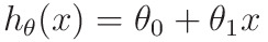
In Vector Form:

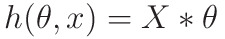
m -> number of elements in the dataset
X -> mx2 matrix
θ -> 2x1 matrix
m -> dataset size
Outputs mx2 matrix

Vector Form is implemented here for faster Operation.

def hypothesis(x, theta):
    '''calculates the hypothesis function'''
    return np.matmul(x, theta)

Cost Function

This essentially calculates the distance between what we need the line to be, and what it actually is:

Definition:
- m -> number of elements in the dataset
- x⁽ⁱ⁾ -> value of x in i^th data point
- y⁽ⁱ⁾ -> value of y in i^th data point

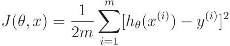
Vector Form for faster implementation
- m -> number of elements in the dataset
- h(θ, X) and Y -> mx1 matrix
- Outputs 1x1 matrix

def compute_cost(x, y, theta):
    '''outputs the cost function'''
    m = len(y)
    error = hypothesis(x, theta) - y
    error_square_summed = np.matmul(np.transpose(error), error)
    return 1/(2*m)*error_square_summed

Gradient Descent

Gradient Descent is an iterative way through which we can minimize the cost function J(θ,x), which essentially depends on the values of θ₀ and θ₁

Gradient Descent is implemented as follows:

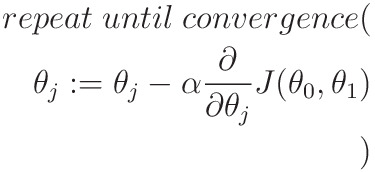
where

α -> a constant, also called learning rate of algorithm
θ_j -> j^th value of θ
J( θ₀ , θ₁ ) -> The Cost Function

This algorithm iteratively minimizes J(θ ,x) to reach it's minimum possible value

Vector Implementation to speed up Algorithm:
- m -> dataset size
- X -> mx2 matrix
- h(θ, X) and Y -> mx1 matrix

def gradient_descent(x, y, theta, alpha, num_iter):
    '''Performs Gradient Descent and outputs minimized theta and history of cost_functions'''
    m = len(y)
    J_history = np.zeros((num_iter, 1))

    for iter in range(num_iter):
        h = hypothesis(x, theta)
        error = h-y
        partial_derivative = 1/m * np.matmul(np.transpose(x), error)
        theta = theta - alpha*partial_derivative

        J_history[iter] = compute_cost(x, y, theta)

    return theta, J_history

Predict

uses hypothesis() to predict value of new input

def predict(value, theta):
    x_array = [1, value]
    return hypothesis(x_array,theta)

Now Let's start the actual processing

Processing

Loading Data from ex1data1.txt

In each line, first value is 'Population of City in 10,000s' and second value is 'Profit in $10,000s'

data_path = "./ex1data1.txt"
data = np.loadtxt(data_path, delimiter=',')

Extracting Population and Profits from data

# first value is independent variable x, second is dependant y
independent_x = data[:, 0]
dependant_y = data[:, 1]

Plotting the Scatter-Plot of data

# showing data
print("Plotting Data ...\n")
plt.figure("Scatter Plot Visualization of Data")
plt.title("Scatter Plot Visualization of Data")
plt.scatter(independent_x, dependant_y, marker="x", c="r")
plt.ylabel('Profit in $10,000s')
plt.xlabel('Population of City in 10,000s')

These lines of codes output this graph

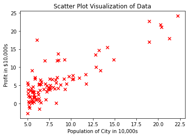
Converting x and y in matrix form

as x and y are 1D vector, they have to converted to their respective matrix form

Also as we are about to do a Matrix Multiplication, to simulate h_θ(x) = θ₀ + θ₁ * x , we are appending 1 to every rows of x to simulate addition of θ₀ by matrix multiplication.

# as we are going to use matrix multiplication, we need x as first column 1, second column values
dataset_size = independent_x.shape[0]
ones = np.ones(dataset_size)
x = np.stack((ones, independent_x), axis=1)

# also converting y in vector form to matrix form
y = dependant_y.reshape(len(dependant_y), 1)

Testing hypothesis and cost function with sample inputs

# initializing theta
theta = np.zeros((2, 1))
alpha = 0.01
num_iter = 1500

print("Testing the cost function ...")
print(f"with theta = [[0],[0]] \nCost computed = {compute_cost(x,y,theta)}")
print("Expected cost value (approx) 32.07\n")

print(f"with theta = [[-1],[2]] \nCost computed = {compute_cost(x,y,[[-1],[2]])}")
print("Expected cost value (approx) 54.24\n")

Running Gradient Descent

print("Running Gradient Descent ...\n")
minimized_theta, J_history = gradient_descent(x, y, theta, alpha, num_iter)

Plotting Value of J during Gradient Descent

If there is value of α is not high, this should decrease with epochs

plt.figure("Value of J during Gradient Descent")
plt.title('Value of J during Gradient Descent')
x_axis = range(len(J_history))
plt.xlabel('No. of iterations or Epochs')
plt.ylabel("Cost function J")
plt.plot(x_axis,J_history)

A sample graph generated from this...

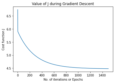
Testing Minimized Theta

print("Theta found by gradient descent:")
print(minimized_theta)
print("Expected theta values (approx)")
print("  3.6303\n  1.1664\n")

Predicting Value for new Inputs

print(f"For population = 35,000, we predict a profit of {predict(3.5, minimized_theta)*10000}")
print(f"For population = 70,000, we predict a profit of {predict(7, minimized_theta)*10000}")

Plotting Scatterplot and the Line of Hypothesis

plt.figure("Linear Regression Result")
plt.title("Linear Regression Result")
plt.scatter(independent_x, dependant_y, marker="x", c="r")
plt.plot(x[:, 1], hypothesis(x, minimized_theta))
plt.ylabel('Profit in $10,000s')
plt.xlabel('Population of City in 10,000s')
plt.show()

A Sample graph from the above code...

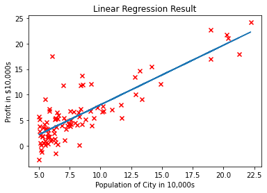
Conclusion

I have linked a .ipynb file Here, if you want to see the code in action, do note that the dataset will not be accessible if you will open the file in colab, you have to download that from Here (This dataset is taken from the Course Assignment)

Here is a Link to the Machine Learning Course I was talking about...

Hope You Have Liked The Document 😁

Linear Regression with Multiple Variable

This is the python version of Linear Regression, most of this is converted from octave/matlab code of the Stanford Machine Learning Course from Coursera

This will be purely Mathematical and Algorithmic

Importing required libraries...

import numpy as np
import matplotlib.pyplot as plt

Functions to be used...

Let's first define the functions that will be called in actual code...

Hypothesis function

Outputs Y, Given X, by parameter θ

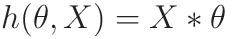
m -> number of elements in the dataset
n -> no. of features of a data (in this example 2)
X -> m x (n+1) matrix
- +1 as we have concatenated 1 so as to keep θ₀ as constant
θ -> (n+1) x 1 matrix
Outputs mx1 matrix

def hypothesis(x, theta):
    '''calculates the hypothesis function'''
    return np.matmul(x, theta)

Cost Function

This essentially calculates the distance between what we need the line to be, and what it actually is:

Vector Form for faster implementation
- m -> number of elements in the dataset
- h(θ, X) and Y -> mx1 matrix
- Outputs 1x1 matrix

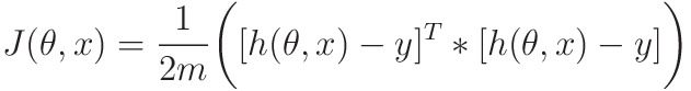
def compute_cost(x, y, theta):
    '''outputs the cost function'''
    m = len(y)
    error = hypothesis(x, theta) - y
    error_square_summed = np.matmul(np.transpose(error), error)
    return 1/(2*m)*error_square_summed

Gradient Descent

Gradient Descent is an iterative way through which we can minimize the cost function J(θ,x), which essentially depends on the values of θ₀ and θ₁

This algorithm iteratively minimizes J(θ ,x) to reach it's minimum possible value

Vector Implementation to speed up Algorithm:
- m -> dataset size
- n -> no. of features of a data (in this example 2)
- X -> m x (n+1) matrix
- h(θ, X) and Y -> mx1 matrix
- θ -> (n+1) x 1 matrix

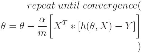
def gradient_descent(x, y, theta, alpha, num_iter):
    '''Performs Gradient Descent and outputs minimized theta and history of cost_functions'''
    m = len(y)
    J_history = np.zeros((num_iter, 1))

    for iter in range(num_iter):
        h = hypothesis(x, theta)
        error = h-y
        partial_derivative = 1/m * np.matmul(np.transpose(x), error)
        theta = theta - alpha*partial_derivative

        J_history[iter] = compute_cost(x, y, theta)

    return theta, J_history

Normalization

As Features of X might be skewed, it is safer to normalize the features of X to same range, this reduces error, and also make learning faster

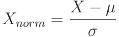
X -> m x n matrix (note there is no +1)
μ -> 1 x n matrix, mean of the features of X
σ -> 1 x n matrix, standard deviation of the features of X

This essentially converts all values of a feature in the range (-1,1)

def featureNormalize(X):
    mu = np.mean(X,axis=0)
    sigma = np.std(X,axis=0)
    X_norm = (X-mu)/sigma
    return X_norm,mu,sigma

Predict

Uses hypothesis() to predict value of new input

def predict(value, minimized_theta,mu,sigma):
    value = np.array(value)
    mu = np.array(mu)
    sigma = np.array(sigma)


    mu = mu.reshape(1,mu.shape[0])
    sigma = sigma.reshape(1,sigma.shape[0])

    normalized_value =  (value -mu)/sigma
    one = np.array([[1]])
    x_array = np.concatenate((one,normalized_value),axis=1)
    return hypothesis(x_array,minimized_theta)

Processing

Loading Data from ex1data2.txt

The ex1data2.txt contains a training set of housing prices in Port- land, Oregon. The first column is the size of the house (in square feet), the second column is the number of bedrooms, and the third column is the price of the house.

data_path = "./ex1data2.txt"
data = np.loadtxt(data_path, delimiter=',')

Extracting Population and Profits from data

# first value is independent variable x, second is dependant y
X= data[:, 0:2]
Y = data[:, 2]

Printing Some Data Points

print("First 10 examples from the dataset")

for iter in range(10):
    print(f"X = {X[iter]}, Y = {Y[iter]}")

Normalizing

By looking in the value of X, we see that value are not in same range, so we normalize the value of X so that the learning becomes more accurate and fast

while predicting, model will give normalized output, we need to de-normalize it

X,mu,sigma = featureNormalize(X)

Adding ones to X and changing y from vector to 2D array

#adding ones to X
dataset_size = X.shape[0]
ones = np.ones(dataset_size).reshape(dataset_size,1)
X = np.concatenate((ones,X),axis=1)

Y = Y.reshape(dataset_size,1)

print(X.shape)

Running Gradient Descent

print("Running Gradient Descent ...\n")
alpha = 1
num_iter = 10
theta = np.zeros((X.shape[1],1))
minimized_theta, J_history = gradient_descent(X, Y, theta, alpha, num_iter)

print("Theta found by gradient descent:")
print(minimized_theta)

Plotting Value of J during Gradient Descent

This should Decrease with Epochs

plt.figure("Value of J during Gradient Descent")
plt.title('Value of J during Gradient Descent')
x_axis = range(len(J_history))
plt.xlabel('No. of iterations or Epochs')
plt.ylabel("Cost function J")
plt.plot(x_axis,J_history)

This will give a graph like this...

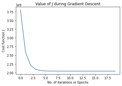
Estimate

Estimate the price of a 1650 sq-ft, 3 bedroom house

predict_input = np.array([1650,3])
predict_input = predict_input.reshape(1,predict_input.shape[0])

print(f"Predicted Price of a 1650 sq-ft, 3 bedroom house: {predict(predict_input,minimized_theta,mu,sigma)}")

Deep Learning

Deep Learning is a Subset of Machine Learning, which specializes in using the concept of Artificial intelligence to solve Real Life Problems.

Topics Covered

Neural Network

Neural Network

Neural Network is a series of algorithm which works together to solve a problem by mimicking what a Human Brain would do if put into that same situation.

Before going into more detail of how actual Neural Networks are implemented, let us discuss how our brain works...

How a Human Brain Works

To put it in a simple way, Human Brain is a collection of a lot of connected Neurons

Here is a Photo of a neuron in brain (Source)

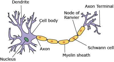
You can think of the parts of a Neuron as follows:

Dendrite: The place from where the Neuron Takes Input
Cell Body: The Place where Neuron processes the Input
Axon: The Place where the Neuron give it's processed data to next Neuron

Believe it or not, but billions of neurons in you brain works together, to do what we all do.

These Neurons are not so much specialized on what they do (although their collection are, but that is related to Biology) but together they adapt to whatever that is needed to be learnt.

For Example, Researchers at MIT once rewired the Auditory Cortex (the part which make us 'hear'), to the eyes, and the Auditory Cortex itself learnt how to see. For more information, click Here.

So it is believed that same things happen in a Neuron, no matter whats it's supposed to do. This is what is mimicked in Artificial Neural Network.

Artificial Neural Network

An Artificial Neural Network is a collection of "Node" connected together to solve a problem.

Here is a sample image of a Artificial Neural Network (Source)

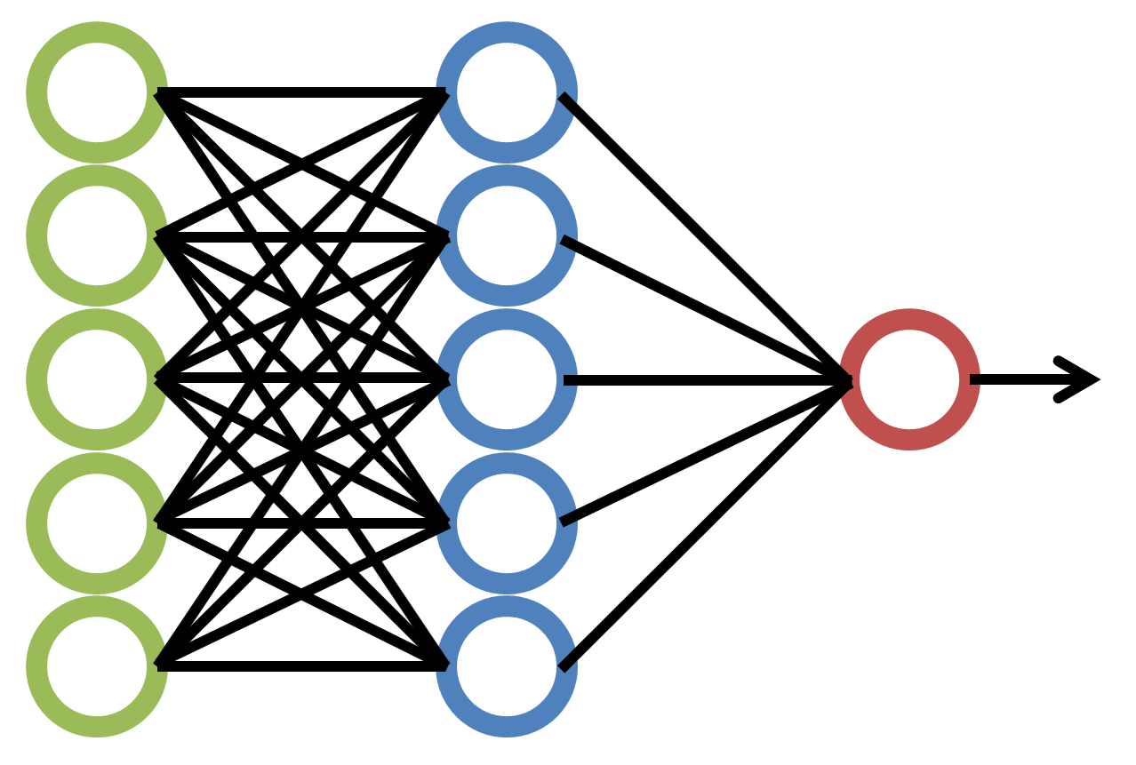
Following things are Important to note in the above Diagram:

All Circles are called node in the Artificial Neural Network. They Take Inputs, Process them, and give their outputs to the next node
The Green nodes are called Input Nodes,
- They take input directly from the data to be learned, process them, and give their output to the next layer.
- There can only be one Input Layer
- All input node collectively takes a vector as input
The Blue Nodes are called Hidden Layer
- They inputs from all the nodes from their previous layer, process them, and gives the output to next layer.
- There can be many hidden layers
The Red node is called the Output Layer
- They take input from their previous layer, process them, and give an output, which says what the Neural Network has "thought" of the input given to it.
The concept of nodes are just for easier understanding. In algorithm, they are implemented as mathematical formulas
All the arrows here are called "data transfer" in algorithm, they are called the learning parameters. The Machine trains itself by tuning these parameters.
This type of model is called a Sequential Model, and the layers are called Dense Layers.

Where to use this model

This model may solve any problem, which are coded with traditional programming,but they are not used there as they have to be trained to work as intended, which might take a long time to do.

These class of models are used to process the things, which are not easily done by traditional programming methods.

Before moving further let's look at another topic

Image

What does Image has to do with Machine Learning?

Image is one of the popular data, where it's very hard to implement Traditional Programming Methods, This is one of the places where the Neural Network Model Shines.

Before discussing why the Neural Network shines here, lets look why it doesn't work well with traditional programming...

Image is an object which gives us an visual representation of something

Let's take an example of the above image of Neural Network, A human sees it at circles connected via line (for simplicity).

But computer perceives it as follows:

A 2D matrix of a 3 number set, which signifies the color at a specific point
Each 3 set number is called a pixel

There are many types of Image representation, some of them are:

RGB Image
- Pixel are a set of three numbers, which signifies intensity of Red, Green, and Blue color in the scale of 0-255
Binary Image
- Pixel is a single number, which is either 0 for white and 1 for black
Greyscale Image
- Pixel is a single number ranging from 0-255 which signifies the intensity of black, which 255 being pure black
- This image is commonly called black and white image (yes, I know it's confusing)

You might wonder why the value 255 is coming so much, this is because generally a pixel is represented by a 8 bit number (or 8*3 for rgb). Nowadays 10 bit colors are also emerging, which can display a lot of numbers than an 8 bit image. This is called bit depth and to know more, see this Video

Machine Learning with TensorFlow

With All the Introduction out of the way, let's start to understand how to actually implement this Machine using TensorFlow 2

TensorFlow 2 is a open-source platform of Machine Learning, and we can use it to develop Machine Learning Model with relatively less amount of codes than pure mathematical execution. This make it easy for us to understand what's actually happening in big picture, rather than delving into complex mathematical operations. To know more about this platform, Click Here

Along with TensorFlow we also use Matplotlib for Plotting Graphs to Better Understand what's actually going on...

To know more about Matplotlib, click here

We will be working on MNIST Dataset, This dataset has 70000 data of 28x28 matrices, which is an image of a digit from 0-9

Here is a sample image from the dataset

Importing Dataset

This dataset is so common that it's readily available inside the tensorFlow module itself and can be loaded in as follows

    from tensorflow.keras.datasets import mnist
    (x_train,y_train), (x_valid,y_valid) = mnist.load_data()

This automatically downloads dataset and divides it into Training and Validation Dataset

Training Dataset is the part by which, the Machine trains itself, and Validation dataset is the part by which we test how good is the prediction of the machine.

y values are the labels, which tells which digit is it's corresponding x

Exploring Dataset

We can see the shape of the Training and validation Dataset by the following code...

print(x_train.shape)

This will print (60000, 28, 28), signifying that x_train has 60000 dataset, each of them are 28x28 matrix

Here's the code to print the image above:

import matplotlib.pyplot as plt
import random

value = random.randint(0,x_train.shape[0])
plt.axis('off')
plt.imshow(x_train[value],cmap='Greys')
print(y_train[value])

random.randint(a,b) gives a random number between a and b, and plt.imshow(matrix) shows the image, cmap option here decides which color space to use for displaying. To know more about imshow(), click Here

Flattening Dataset

The Machine can't take 28x28 array as an input, as we saw that it takes a Vector or 1D array as input. So we reshape them to 784 element 1D array (28*28 = 784), by the following code...

x_train = x_train.reshape(x_train.shape[0],x_train.shape[1]*x_train.shape[2])
x_valid = x_valid.reshape(x_valid.shape[0],x_valid.shape[1]*x_valid.shape[2])

print(x_train.shape)
print(x_valid.shape)

This will print (60000, 784) and (10000, 784), signifying that 28x28 2D matrix has been converted to 784 1D matrix. This is called flattening the images.

Normalizing Dataset

The TensorFlow model, which we are going to use requires input values to be in the range 0-1, so we need to convert the images range 0-255 to 0-1, we do it by the following...

x_train = x_train / 255
x_valid = x_valid / 255

This step is called Normalization

Categorical Encoding

The y_train and y_valid are a number ranging from 0-9 , but as the model will be working in float values between 0 and 1, and can only give outputs in that range, so what we do is that we convert y_train and y_valid to a set of 10 numbers with following property

i^th value of y_train will be 1 if y_train was i

This was super simplified as only one data point was in question, in reality we have to convert an n size dataset of output to nxm size dataset, where m is the max value of y. This is called Categorical Encoding.

Luckily TensorFlow has built-in function to_categorical for this, which is done by following code...

import tensorflow.keras as keras

num_category = 10

y_train = keras.utils.to_categorical(y_train,num_category)
y_valid = keras.utils.to_categorical(y_valid,num_category)

Now we have the data set up as needed, we can now proceed to building the model...

Building the Model

The Build will be as follows:

We build a Sequential Model
784 nodes for input layer
A single hidden layer with 512 nodes
10 outputs layers each having a probability that what digit it is
All layers will be Dense

All this can be done in the following codes

from tensorflow.keras.models import Sequential
from tensorflow.keras.layers import Dense

model = Sequential()


model.add(Dense(units=784,activation='relu',input_shape=(784,)))
model.add(Dense(units=512,activation='relu'))
model.add(Dense(units=10,activation='softmax'))

model.compile(loss='categorical_crossentropy',metrics=['accuracy'])

Here the words relu, softmax, and categorical_crossentropy are purely mathematical terms, which I will not be explaining right now, I you wanna know more about ReLu, Softmax, and Categorical Cross-Entropy, click the respective links.

What I will say that softmax makes sure that outputs nodes will be probabilistic value, i.e sum of all the output node's output will be one. This makes determining the best guess easier than not using softmax.

Training the Model

The Model Formed can be trained by the following code...

history = model.fit(x_train,y_train,epochs=20,verbose=1,validation_data=(x_valid,y_valid))

Here epochs means number of time to train the model, One Epoch means a full pass of the data set.

This Outputs history, which contains all the evaluation parameters for all the epochs.

Analyzing Output

we can find what data history has by following...

history.history.keys()

This Outputs dict_keys(['loss', 'accuracy', 'val_loss', 'val_accuracy']), which says that history.history is a dictionary data structure with the given four parameters.

To plot the data in history, we do the following...

import matplotlib.pyplot as plt

fig,(ax1,ax2) = plt.subplots(1,2)
fig.set_size_inches(20,8)

fig.suptitle('Metrics Of Neural Network')

ax1.plot(history.history['loss'])
ax1.plot(history.history['val_loss'])
ax1.legend(['loss','val_loss'])
ax1.set_title('Loss')

ax2.plot(history.history['accuracy'])
ax2.plot(history.history['val_accuracy'])
ax2.legend(['accuracy','val_accuracy'])
ax2.set_title('Accuracy')

This Shows the following two graphs...

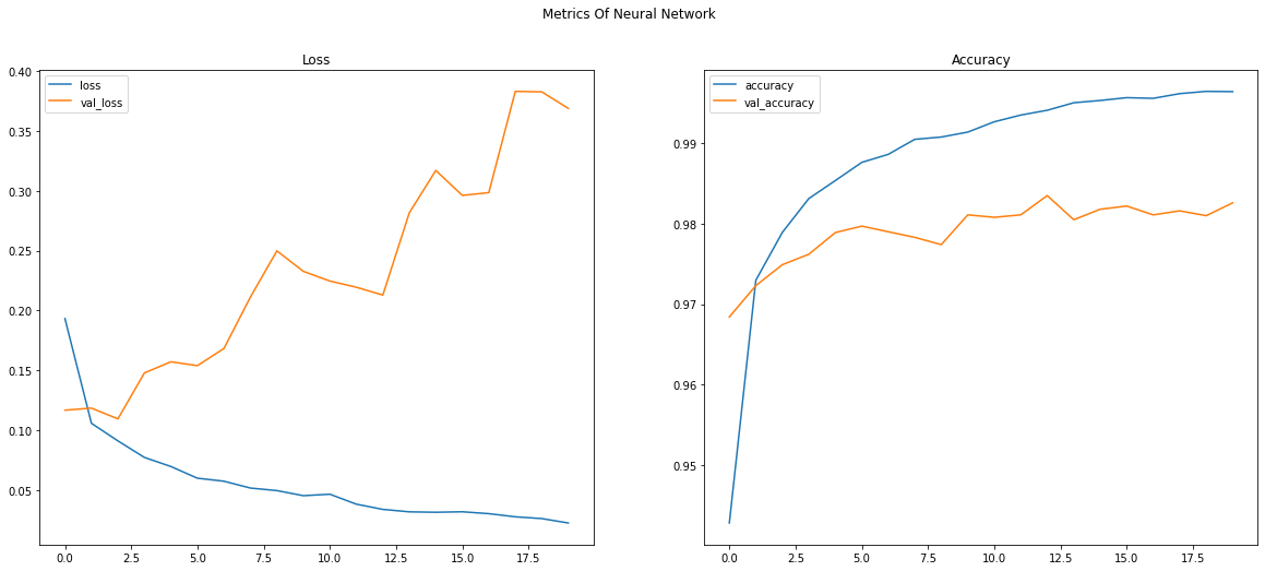
Here we see that as the epochs gets continued, although training loss keeps getting decreased and training accuracy keeps increasing (the blue lines), the Validation Loss keep increasing, and Validation Accuracy keeps decreasing.

This means that the model will give very good results with the models he has already seen, but perform poorly on new data. This is a very bad thing and should be avoided. This is called the Problem of Overfitting.

Conclusion

I have also provided a .ipynb file here, I you wanna see the codes in action.

Hope you have found my guide informative. 😄