Linear Regression with one Variable
This is the python version of Linear Regression, most of this is converted from octave/matlab code of the Stanford Machine Learning Course from Coursera
This will be purely Mathematical and Algorithmic
Importing required libraries...
import numpy as np
import matplotlib.pyplot as plt
Functions to be used...
Let's first define the functions that will be called in actual code...
Hypothesis function
Outputs Y, Given X, by parameter θ
- In Simple Definition:
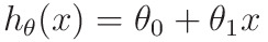
- In Vector Form:
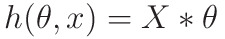
- m -> number of elements in the dataset
- X -> mx2 matrix
- θ -> 2x1 matrix
- m -> dataset size
- Outputs mx2 matrix
Vector Form is implemented here for faster Operation.
def hypothesis(x, theta):
    '''calculates the hypothesis function'''
    return np.matmul(x, theta)
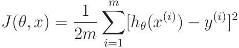
Cost Function
This essentially calculates the distance between what we need the line to be, and what it actually is:
- Definition:
- m -> number of elements in the dataset
- x(i) -> value of x in ith data point
- y(i) -> value of y in ith data point
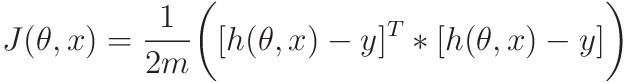
- Vector Form for faster implementation
- m -> number of elements in the dataset
- h(θ, X) and Y -> mx1 matrix
- Outputs 1x1 matrix
def compute_cost(x, y, theta):
    '''outputs the cost function'''
    m = len(y)
    error = hypothesis(x, theta) - y
    error_square_summed = np.matmul(np.transpose(error), error)
    return 1/(2*m)*error_square_summed
Gradient Descent
Gradient Descent is an iterative way through which we can minimize the cost function J(θ,x), which essentially depends on the values of θ0 and θ1
Gradient Descent is implemented as follows:
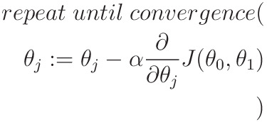
where
- α -> a constant, also called learning rate of algorithm
- θj -> jth value of θ
- J( θ0 , θ1 ) -> The Cost Function
This algorithm iteratively minimizes J(θ ,x) to reach it's minimum possible value
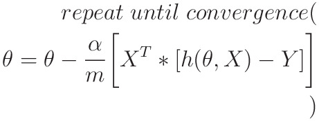
- Vector Implementation to speed up Algorithm:
- m -> dataset size
- X -> mx2 matrix
- h(θ, X) and Y -> mx1 matrix
def gradient_descent(x, y, theta, alpha, num_iter):
    '''Performs Gradient Descent and outputs minimized theta and history of cost_functions'''
    m = len(y)
    J_history = np.zeros((num_iter, 1))

    for iter in range(num_iter):
        h = hypothesis(x, theta)
        error = h-y
        partial_derivative = 1/m * np.matmul(np.transpose(x), error)
        theta = theta - alpha*partial_derivative

        J_history[iter] = compute_cost(x, y, theta)

    return theta, J_history
Predict
uses hypothesis() to predict value of new input
def predict(value, theta):
    x_array = [1, value]
    return hypothesis(x_array,theta)
Now Let's start the actual processing
Processing
Loading Data from ex1data1.txt
In each line, first value is 'Population of City in 10,000s' and second value is 'Profit in $10,000s'
data_path = "./ex1data1.txt"
data = np.loadtxt(data_path, delimiter=',')
Extracting Population and Profits from data
# first value is independent variable x, second is dependant y
independent_x = data[:, 0]
dependant_y = data[:, 1]
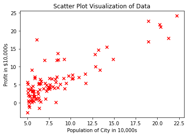
Plotting the Scatter-Plot of data
# showing data
print("Plotting Data ...\n")
plt.figure("Scatter Plot Visualization of Data")
plt.title("Scatter Plot Visualization of Data")
plt.scatter(independent_x, dependant_y, marker="x", c="r")
plt.ylabel('Profit in $10,000s')
plt.xlabel('Population of City in 10,000s')
These lines of codes output this graph
Converting x and y in matrix form
as x and y are 1D vector, they have to converted to their respective matrix form
Also as we are about to do a Matrix Multiplication, to simulate hθ(x) = θ0 + θ1 * x , we are appending 1 to every rows of x to simulate addition of θ0 by matrix multiplication.
# as we are going to use matrix multiplication, we need x as first column 1, second column values
dataset_size = independent_x.shape[0]
ones = np.ones(dataset_size)
x = np.stack((ones, independent_x), axis=1)

# also converting y in vector form to matrix form
y = dependant_y.reshape(len(dependant_y), 1)
Testing hypothesis and cost function with sample inputs
# initializing theta
theta = np.zeros((2, 1))
alpha = 0.01
num_iter = 1500

print("Testing the cost function ...")
print(f"with theta = [[0],[0]] \nCost computed = {compute_cost(x,y,theta)}")
print("Expected cost value (approx) 32.07\n")

print(f"with theta = [[-1],[2]] \nCost computed = {compute_cost(x,y,[[-1],[2]])}")
print("Expected cost value (approx) 54.24\n")
Running Gradient Descent
print("Running Gradient Descent ...\n")
minimized_theta, J_history = gradient_descent(x, y, theta, alpha, num_iter)
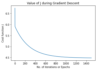
Plotting Value of J during Gradient Descent
If there is value of α is not high, this should decrease with epochs
plt.figure("Value of J during Gradient Descent")
plt.title('Value of J during Gradient Descent')
x_axis = range(len(J_history))
plt.xlabel('No. of iterations or Epochs')
plt.ylabel("Cost function J")
plt.plot(x_axis,J_history)
A sample graph generated from this...
Testing Minimized Theta
print("Theta found by gradient descent:")
print(minimized_theta)
print("Expected theta values (approx)")
print("  3.6303\n  1.1664\n")
Predicting Value for new Inputs
print(f"For population = 35,000, we predict a profit of {predict(3.5, minimized_theta)*10000}")
print(f"For population = 70,000, we predict a profit of {predict(7, minimized_theta)*10000}")
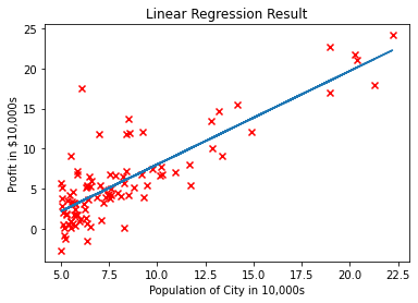
Plotting Scatterplot and the Line of Hypothesis
plt.figure("Linear Regression Result")
plt.title("Linear Regression Result")
plt.scatter(independent_x, dependant_y, marker="x", c="r")
plt.plot(x[:, 1], hypothesis(x, minimized_theta))
plt.ylabel('Profit in $10,000s')
plt.xlabel('Population of City in 10,000s')
plt.show()
A Sample graph from the above code...
Conclusion
I have linked a .ipynb file Here, if you want to see the code in action, do note that the dataset will not be accessible if you will open the file in colab, you have to download that from Here (This dataset is taken from the Course Assignment)
Here is a Link to the Machine Learning Course I was talking about...
Hope You Have Liked The Document 😁