Linear Regression with Multiple Variable

This is the python version of Linear Regression, most of this is converted from octave/matlab code of the Stanford Machine Learning Course from Coursera

This will be purely Mathematical and Algorithmic

Importing required libraries...

import numpy as np
import matplotlib.pyplot as plt

Functions to be used...

Let's first define the functions that will be called in actual code...

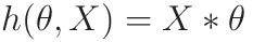
Hypothesis function

Outputs Y, Given X, by parameter θ

m -> number of elements in the dataset
n -> no. of features of a data (in this example 2)
X -> m x (n+1) matrix
- +1 as we have concatenated 1 so as to keep θ₀ as constant
θ -> (n+1) x 1 matrix
Outputs mx1 matrix

def hypothesis(x, theta):
    '''calculates the hypothesis function'''
    return np.matmul(x, theta)

Cost Function

This essentially calculates the distance between what we need the line to be, and what it actually is:

Vector Form for faster implementation
- m -> number of elements in the dataset
- h(θ, X) and Y -> mx1 matrix
- Outputs 1x1 matrix

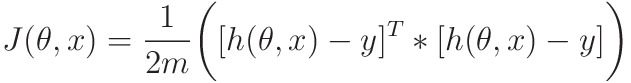
def compute_cost(x, y, theta):
    '''outputs the cost function'''
    m = len(y)
    error = hypothesis(x, theta) - y
    error_square_summed = np.matmul(np.transpose(error), error)
    return 1/(2*m)*error_square_summed

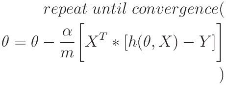
Gradient Descent

Gradient Descent is an iterative way through which we can minimize the cost function J(θ,x), which essentially depends on the values of θ₀ and θ₁

This algorithm iteratively minimizes J(θ ,x) to reach it's minimum possible value

Vector Implementation to speed up Algorithm:
- m -> dataset size
- n -> no. of features of a data (in this example 2)
- X -> m x (n+1) matrix
- h(θ, X) and Y -> mx1 matrix
- θ -> (n+1) x 1 matrix

def gradient_descent(x, y, theta, alpha, num_iter):
    '''Performs Gradient Descent and outputs minimized theta and history of cost_functions'''
    m = len(y)
    J_history = np.zeros((num_iter, 1))

    for iter in range(num_iter):
        h = hypothesis(x, theta)
        error = h-y
        partial_derivative = 1/m * np.matmul(np.transpose(x), error)
        theta = theta - alpha*partial_derivative

        J_history[iter] = compute_cost(x, y, theta)

    return theta, J_history

Normalization

As Features of X might be skewed, it is safer to normalize the features of X to same range, this reduces error, and also make learning faster

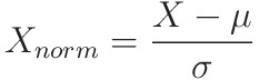
X -> m x n matrix (note there is no +1)
μ -> 1 x n matrix, mean of the features of X
σ -> 1 x n matrix, standard deviation of the features of X

This essentially converts all values of a feature in the range (-1,1)

def featureNormalize(X):
    mu = np.mean(X,axis=0)
    sigma = np.std(X,axis=0)
    X_norm = (X-mu)/sigma
    return X_norm,mu,sigma

Predict

Uses hypothesis() to predict value of new input

def predict(value, minimized_theta,mu,sigma):
    value = np.array(value)
    mu = np.array(mu)
    sigma = np.array(sigma)


    mu = mu.reshape(1,mu.shape[0])
    sigma = sigma.reshape(1,sigma.shape[0])

    normalized_value =  (value -mu)/sigma
    one = np.array([[1]])
    x_array = np.concatenate((one,normalized_value),axis=1)
    return hypothesis(x_array,minimized_theta)

The ex1data2.txt contains a training set of housing prices in Port- land, Oregon. The first column is the size of the house (in square feet), the second column is the number of bedrooms, and the third column is the price of the house.

data_path = "./ex1data2.txt"
data = np.loadtxt(data_path, delimiter=',')

Extracting Population and Profits from data

# first value is independent variable x, second is dependant y
X= data[:, 0:2]
Y = data[:, 2]

Printing Some Data Points

print("First 10 examples from the dataset")

for iter in range(10):
    print(f"X = {X[iter]}, Y = {Y[iter]}")

Normalizing

By looking in the value of X, we see that value are not in same range, so we normalize the value of X so that the learning becomes more accurate and fast

while predicting, model will give normalized output, we need to de-normalize it

X,mu,sigma = featureNormalize(X)

Adding ones to X and changing y from vector to 2D array

#adding ones to X
dataset_size = X.shape[0]
ones = np.ones(dataset_size).reshape(dataset_size,1)
X = np.concatenate((ones,X),axis=1)

Y = Y.reshape(dataset_size,1)

print(X.shape)

Running Gradient Descent

print("Running Gradient Descent ...\n")
alpha = 1
num_iter = 10
theta = np.zeros((X.shape[1],1))
minimized_theta, J_history = gradient_descent(X, Y, theta, alpha, num_iter)

print("Theta found by gradient descent:")
print(minimized_theta)

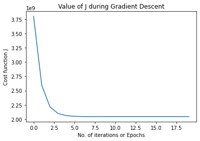
Plotting Value of J during Gradient Descent

This should Decrease with Epochs

plt.figure("Value of J during Gradient Descent")
plt.title('Value of J during Gradient Descent')
x_axis = range(len(J_history))
plt.xlabel('No. of iterations or Epochs')
plt.ylabel("Cost function J")
plt.plot(x_axis,J_history)

This will give a graph like this...

Estimate

Estimate the price of a 1650 sq-ft, 3 bedroom house

predict_input = np.array([1650,3])
predict_input = predict_input.reshape(1,predict_input.shape[0])

print(f"Predicted Price of a 1650 sq-ft, 3 bedroom house: {predict(predict_input,minimized_theta,mu,sigma)}")

Algorithms